Fitting with constraints#
fitting support constraints, however, different fitters support
different types of constraints. The supported_constraints
attribute shows the type of constraints supported by a specific fitter:
>>> from astropy.modeling import fitting
>>> fitting.LinearLSQFitter.supported_constraints
['fixed']
>>> fitting.TRFLSQFitter.supported_constraints
['fixed', 'tied', 'bounds']
>>> fitting.SLSQPLSQFitter.supported_constraints
['bounds', 'eqcons', 'ineqcons', 'fixed', 'tied']
Fixed Parameter Constraint#
All fitters support fixed (frozen) parameters through the fixed argument
to models or setting the fixed
attribute directly on a parameter.
For linear fitters, freezing a polynomial coefficient means that the
corresponding term will be subtracted from the data before fitting a
polynomial without that term to the result. For example, fixing c0 in a
polynomial model will fit a polynomial with the zero-th order term missing
to the data minus that constant. The fixed coefficients and corresponding terms
are restored to the fit polynomial and this is the polynomial returned from the fitter:
>>> import numpy as np
>>> rng = np.random.default_rng(seed=12345)
>>> from astropy.modeling import models, fitting
>>> x = np.arange(1, 10, .1)
>>> p1 = models.Polynomial1D(2, c0=[1, 1], c1=[2, 2], c2=[3, 3],
...                          n_models=2)
>>> p1
<Polynomial1D(2, c0=[1., 1.], c1=[2., 2.], c2=[3., 3.], n_models=2)>
>>> y = p1(x, model_set_axis=False)
>>> n = (rng.standard_normal(y.size)).reshape(y.shape)
>>> p1.c0.fixed = True
>>> pfit = fitting.LinearLSQFitter()
>>> new_model = pfit(p1, x, y + n)
>>> print(new_model)
Model: Polynomial1D
Inputs: ('x',)
Outputs: ('y',)
Model set size: 2
Degree: 2
Parameters:
     c0         c1                 c2
    --- ------------------ ------------------
    1.0  2.072116176718454   2.99115839177437
    1.0 1.9818866652726403 3.0024208951927585
The syntax to fix the same parameter c0 using an argument to the model
instead of p1.c0.fixed = True would be:
>>> p1 = models.Polynomial1D(2, c0=[1, 1], c1=[2, 2], c2=[3, 3],
...                          n_models=2, fixed={'c0': True})
Bounded Constraints#
Bounded fitting is supported through the bounds arguments to models or by
setting min and max
attributes on a parameter. The following fitters support bounds internally:
The LevMarLSQFitter algorithm uses an unsophisticated
method of handling bounds and is no longer recommended (see
Notes on non-linear fitting for more details).
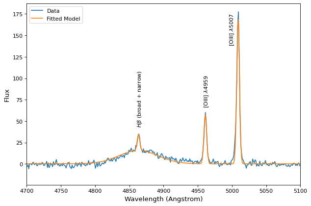
Tied Constraints#
The tied constraint is often useful with
Compound models. In this example we will
read a spectrum from a file called spec.txt and simultaneously fit
Gaussians to the emission lines while linking their wavelengths and
linking the flux of the [OIII] λ4959 line to the [OIII] λ5007 line.
import numpy as np
from astropy.io import ascii
from astropy.modeling import fitting, models
from astropy.utils.data import get_pkg_data_filename
from matplotlib import pyplot as plt

fname = get_pkg_data_filename("data/spec.txt", package="astropy.modeling.tests")
spec = ascii.read(fname)
wave = spec["lambda"]
flux = spec["flux"]

# Use the (vacuum) rest wavelengths of known lines as initial values
# for the fit.
Hbeta = 4862.721
O3_4959 = 4960.295
O3_5007 = 5008.239

# Create Gaussian1D models for each of the H-beta and [OIII] lines.
hbeta_broad = models.Gaussian1D(amplitude=15, mean=Hbeta, stddev=20)
hbeta_narrow = models.Gaussian1D(amplitude=20, mean=Hbeta, stddev=2)
o3_4959 = models.Gaussian1D(amplitude=70, mean=O3_4959, stddev=2)
o3_5007 = models.Gaussian1D(amplitude=180, mean=O3_5007, stddev=2)

# Create a polynomial model to fit the continuum.
mean_flux = flux.mean()
cont = np.where(flux > mean_flux, mean_flux, flux)
linfitter = fitting.LinearLSQFitter()
poly_cont = linfitter(models.Polynomial1D(1), wave, cont)

# Create a compound model for the four emission lines and the continuum.
model = hbeta_broad + hbeta_narrow + o3_4959 + o3_5007 + poly_cont

# Tie the ratio of the intensity of the two [OIII] lines.
def tie_o3_ampl(model):
    return model.amplitude_3 / 2.98

o3_4959.amplitude.tied = tie_o3_ampl

# Tie the wavelengths of the two [OIII] lines
def tie_o3_wave(model):
    return model.mean_3 * O3_4959 / O3_5007

o3_4959.mean.tied = tie_o3_wave

# Tie the wavelengths of the two (narrow and broad) H-beta lines
def tie_hbeta_wave1(model):
    return model.mean_1

hbeta_broad.mean.tied = tie_hbeta_wave1

# Tie the wavelengths of the H-beta lines to the [OIII] 5007 line
def tie_hbeta_wave2(model):
    return model.mean_3 * Hbeta / O3_5007

hbeta_narrow.mean.tied = tie_hbeta_wave2

# Simultaneously fit all the emission lines and continuum.
fitter = fitting.TRFLSQFitter()
fitted_model = fitter(model, wave, flux)
fitted_lines = fitted_model(wave)

# Plot the data and the fitted model
fig, ax = plt.subplots(figsize=(9, 6))
ax.plot(wave, flux, label="Data")
ax.plot(wave, fitted_lines, color="C1", label="Fitted Model")
ax.legend(loc="upper left")
ax.text(4860, 45, r"$H\beta$ (broad + narrow)", rotation=90)
ax.text(4958, 68, r"[OIII] $\lambda 4959$", rotation=90)
ax.text(4995, 140, r"[OIII] $\lambda 5007$", rotation=90)
ax.set(xlim=(4700, 5100), xlabel="Wavelength (Angstrom)", ylabel="Flux")
plt.show()