Convolution and Filtering (astropy.convolution)#
Introduction#
astropy.convolution provides convolution functions and kernels that offer
improvements compared to the SciPy scipy.ndimage convolution routines,
including:
Proper treatment of NaN values (ignoring them during convolution and replacing NaN pixels with interpolated values)
Both direct and Fast Fourier Transform (FFT) versions
Built-in kernels that are commonly used in Astronomy
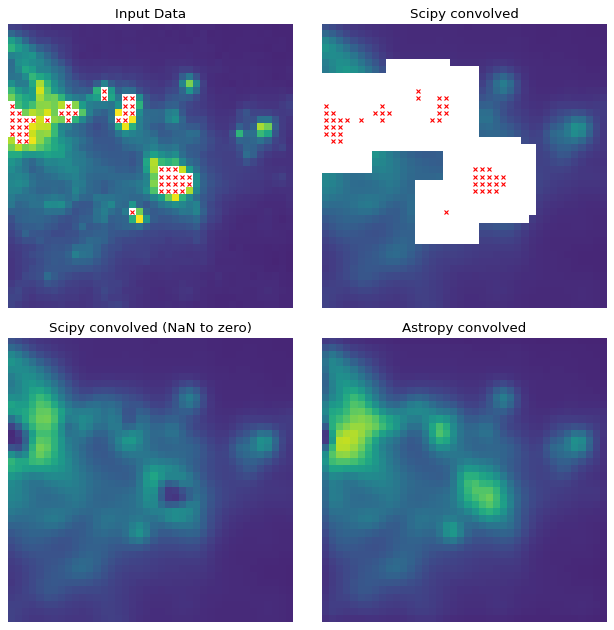
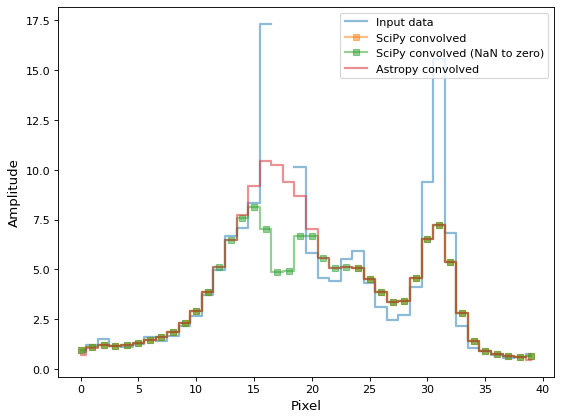
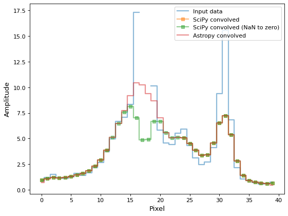
The following thumbnails show the difference between SciPy and Astropy’s convolve functions on an astronomical image that contains NaN values. Scipy’s function returns NaN for all pixels that are within a kernel-sized region of any NaN value, which is often not the desired result.
Getting Started#
Two convolution functions are provided. They are imported as:
from astropy.convolution import convolve, convolve_fft
and are both used as:
result = convolve(image, kernel)
result = convolve_fft(image, kernel)
convolve() is implemented as a direct convolution
algorithm, while convolve_fft() uses a Fast Fourier
Transform (FFT). Thus, the former is better for small kernels, while the latter
is much more efficient for larger kernels.
Example#
To convolve a 1D dataset with a user-specified kernel, you can do:
>>> from astropy.convolution import convolve
>>> convolve([1, 4, 5, 6, 5, 7, 8], [0.2, 0.6, 0.2])
array([1.4, 3.6, 5. , 5.6, 5.6, 6.8, 6.2])
The boundary keyword determines how the input array is extended
beyond its boundaries. The default value is 'fill', meaning values
outside of the array boundary are set to the input fill_value
(default is 0.0). Setting boundary='extend' causes values near the
edges to be extended using a constant extrapolation beyond the boundary.
The values at the end are computed assuming that any value below the
first point is 1, and any value above the last point is 8:
>>> from astropy.convolution import convolve
>>> convolve([1, 4, 5, 6, 5, 7, 8], [0.2, 0.6, 0.2], boundary='extend')
array([1.6, 3.6, 5. , 5.6, 5.6, 6.8, 7.8])
For a more detailed discussion of boundary treatment, see Using the Convolution Functions.
Example#
The convolution module also includes built-in kernels that can be imported as, for example:
>>> from astropy.convolution import Gaussian1DKernel
To use a kernel, first create a specific instance of the kernel:
>>> gauss = Gaussian1DKernel(stddev=2)
gauss is not an array, but a kernel object. The underlying array can be
retrieved with:
>>> gauss.array
array([6.69162896e-05, 4.36349021e-04, 2.21596317e-03, 8.76430436e-03,
       2.69959580e-02, 6.47599366e-02, 1.20987490e-01, 1.76035759e-01,
       1.99474648e-01, 1.76035759e-01, 1.20987490e-01, 6.47599366e-02,
       2.69959580e-02, 8.76430436e-03, 2.21596317e-03, 4.36349021e-04,
       6.69162896e-05])
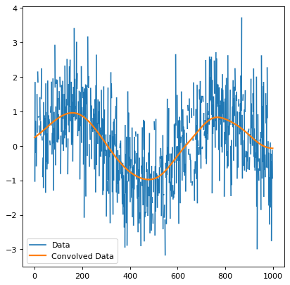
The kernel can then be used directly when calling
convolve():
(Source code, png, svg, pdf)
Using astropy’s Convolution to Replace Bad Data#
astropy’s convolution methods can be used to replace bad data with values
interpolated from their neighbors. Kernel-based interpolation is useful for
handling images with a few bad pixels or for interpolating sparsely sampled
images.
The interpolation tool is implemented and used as:
from astropy.convolution import interpolate_replace_nans
result = interpolate_replace_nans(image, kernel)
Some contexts in which you might want to use kernel-based interpolation include:
Images with saturated pixels. Generally, these are the highest-intensity regions in the imaged area, and the interpolated values are not reliable, but this can be useful for display purposes.
Images with flagged pixels (e.g., a few small regions affected by cosmic rays or other spurious signals that require those pixels to be flagged out). If the affected region is small enough, the resulting interpolation will have a small effect on source statistics and may allow for robust source-finding algorithms to be run on the resulting data.
Sparsely sampled images such as those constructed with single-pixel detectors. Such images will only have a few discrete points sampled across the imaged area, but an approximation of the extended sky emission can still be constructed.
Note
Care must be taken to ensure that the kernel is large enough to completely
cover potential contiguous regions of NaN values.
An AstropyUserWarning is raised if NaN values are detected
post-convolution, in which case the kernel size should be increased.
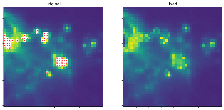
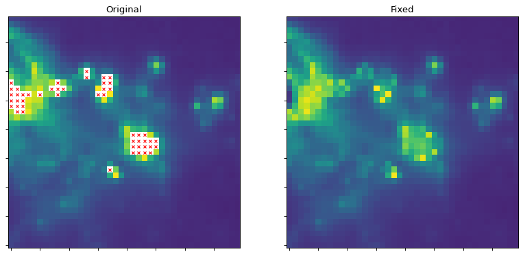
Example#
The script below shows an example of kernel interpolation to fill in flagged-out pixels:
(Source code, png, svg, pdf)
Example#
This script shows the power of this technique for reconstructing images from sparse sampling. Note that the image is not perfect: the pointlike sources are sometimes missed, but the extended structure is very well recovered by eye.


Using astropy.convolution#
Performance Tips#
The convolve() function is best suited to small
kernels, and can become very slow for larger kernels. In this case, consider
using convolve_fft() (though note that this function
uses more memory, and consider the different padding options).