Fitting a Line#
Fitting a line to (x,y) data points is a common case in many areas. Examples fits are given for fitting, fitting using the uncertainties as weights, and fitting using iterative sigma clipping.
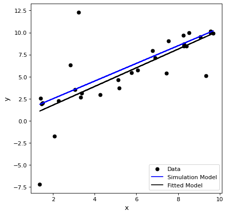
Simple Fit#
Here the (x,y) data points are fit with a line. The (x,y) data points are simulated and have a range of uncertainties to give a realistic example.
import numpy as np
import matplotlib.pyplot as plt
from astropy.modeling import models, fitting

# define a model for a line
line_orig = models.Linear1D(slope=1.0, intercept=0.5)

# generate x, y data non-uniformly spaced in x
# add noise to y measurements
npts = 30
rng = np.random.default_rng(10)
x = rng.uniform(0.0, 10.0, npts)
y = line_orig(x)
yunc = np.absolute(rng.normal(0.5, 2.5, npts))
y += rng.normal(0.0, yunc, npts)

# initialize a linear fitter
fit = fitting.LinearLSQFitter()

# initialize a linear model
line_init = models.Linear1D()

# fit the data with the fitter
fitted_line = fit(line_init, x, y)

# plot
fig, ax = plt.subplots()
ax.plot(x, y, 'ko', label='Data')
ax.plot(x, line_orig(x), 'b-', label='Simulation Model')
ax.plot(x, fitted_line(x), 'k-', label='Fitted Model')
ax.set(xlabel='x', ylabel='y')
ax.legend()
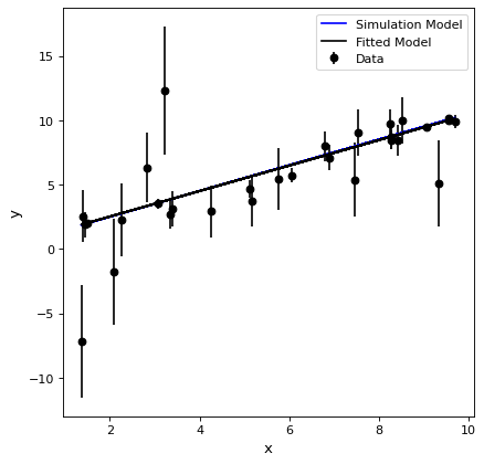
Fit using uncertainties#
Fitting can be done using the uncertainties as weights. To get the standard weighting of 1/unc^2 for the case of Gaussian errors, the weights to pass to the fitting are 1/unc.
import numpy as np
import matplotlib.pyplot as plt
from astropy.modeling import models, fitting

# define a model for a line
line_orig = models.Linear1D(slope=1.0, intercept=0.5)

# generate x, y data non-uniformly spaced in x
# add noise to y measurements
npts = 30
rng = np.random.default_rng(10)
x = rng.uniform(0.0, 10.0, npts)
y = line_orig(x)
yunc = np.absolute(rng.normal(0.5, 2.5, npts))
y += rng.normal(0.0, yunc, npts)

# initialize a linear fitter
fit = fitting.LinearLSQFitter()

# initialize a linear model
line_init = models.Linear1D()

# fit the data with the fitter
fitted_line = fit(line_init, x, y, weights=1.0/yunc)

# plot
fig, ax = plt.subplots()
ax.errorbar(x, y, yerr=yunc, fmt='ko', label='Data')
ax.plot(x, line_orig(x), 'b-', label='Simulation Model')
ax.plot(x, fitted_line(x), 'k-', label='Fitted Model')
ax.set(xlabel='x', ylabel='y')
ax.legend()
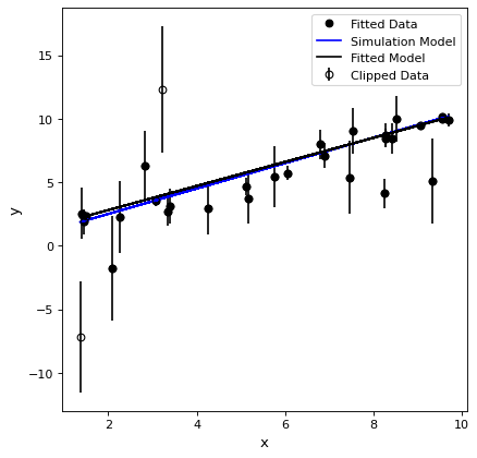
Iterative fitting using sigma clipping#
When fitting, there may be data that are outliers from the fit that can significantly bias the fitting. These outliers can be identified and removed from the fitting iteratively. Note that the iterative sigma clipping assumes all the data have the same uncertainties for the sigma clipping decision.
import numpy as np
import matplotlib.pyplot as plt
from astropy.stats import sigma_clip
from astropy.modeling import models, fitting

# define a model for a line
line_orig = models.Linear1D(slope=1.0, intercept=0.5)

# generate x, y data non-uniformly spaced in x
# add noise to y measurements
npts = 30
rng = np.random.default_rng(10)
x = rng.uniform(0.0, 10.0, npts)
y = line_orig(x)
yunc = np.absolute(rng.normal(0.5, 2.5, npts))
y += rng.normal(0.0, yunc, npts)

# make true outliers
y[3] = line_orig(x[3]) + 6 * yunc[3]
y[10] = line_orig(x[10]) - 4 * yunc[10]

# initialize a linear fitter
fit = fitting.LinearLSQFitter()

# initialize the outlier removal fitter
or_fit = fitting.FittingWithOutlierRemoval(fit, sigma_clip, niter=3, sigma=3.0)

# initialize a linear model
line_init = models.Linear1D()

# fit the data with the fitter
fitted_line, mask = or_fit(line_init, x, y, weights=1.0/yunc)
filtered_data = np.ma.masked_array(y, mask=mask)

# plot
fig, ax = plt.subplots()
ax.errorbar(x, y, yerr=yunc, fmt="ko", fillstyle="none", label="Clipped Data")
ax.plot(x, filtered_data, "ko", label="Fitted Data")
ax.plot(x, line_orig(x), 'b-', label='Simulation Model')
ax.plot(x, fitted_line(x), 'k-', label='Fitted Model')
ax.set(xlabel='x', ylabel='y')
ax.legend()