Time and Dates (astropy.time)#
Introduction#
The astropy.time package provides functionality for manipulating times and
dates. Specific emphasis is placed on supporting time scales (e.g., UTC, TAI,
UT1, TDB) and time representations (e.g., JD, MJD, ISO 8601) that are used in
astronomy and required to calculate, for example, sidereal times and barycentric
corrections. The astropy.time package is based on fast and memory efficient
PyERFA wrappers around the ERFA time and calendar routines.
All time manipulations and arithmetic operations are done internally using two
64-bit floats to represent time. Floating point algorithms from [1] are used so
that the Time object maintains sub-nanosecond precision over times spanning
the age of the universe.
Getting Started#
The usual way to use astropy.time is to create a Time object by
supplying one or more input time values as well as the time format and time
scale of those values. The input time(s) can either be a single scalar like
"2010-01-01 00:00:00" or a list or a numpy array of values as shown
below. In general, any output values have the same shape (scalar or array) as
the input.
Examples#
To create a Time object:
>>> import numpy as np
>>> from astropy.time import Time
>>> times = ['1999-01-01T00:00:00.123456789', '2010-01-01T00:00:00']
>>> t = Time(times, format='isot', scale='utc')
>>> t
<Time object: scale='utc' format='isot' value=['1999-01-01T00:00:00.123' '2010-01-01T00:00:00.000']>
>>> t[1]
<Time object: scale='utc' format='isot' value=2010-01-01T00:00:00.000>
The format argument specifies how to interpret the input values (e.g., ISO,
JD, or Unix time). By default, the same format will be used to represent the
time for output. One can change this format later as needed, but because this
is just for representation, that does not affect the internal representation
(which is always by two 64-bit values, the jd1 and jd2 attributes), nor
any computations with the object.
The scale argument specifies the time scale for the values
(e.g., UTC, TT, or UT1). The scale argument is optional and defaults
to UTC except for Time from Epoch Formats. It is possible to change
it (e.g., from UTC to TDB), which will cause the internal values to be
adjusted accordingly.
We could have written the above as:
>>> t = Time(times, format='isot')
When the format of the input can be unambiguously determined, the
format argument is not required, so we can then simplify even further:
>>> t = Time(times)
Now we can get the representation of these times in the JD and MJD
formats by requesting the corresponding Time attributes:
>>> t.jd
array([2451179.50000143, 2455197.5       ])
>>> t.mjd
array([51179.00000143, 55197.        ])
The full power of output representation is available via the
to_value method which also allows controlling the
subformat. For instance, using numpy.longdouble as the output type
for higher precision:
>>> t.to_value('mjd', 'long')
array([51179.00000143, 55197.        ], dtype=float128)
The default representation can be changed by setting the format attribute:
>>> t.format = 'fits'
>>> t
<Time object: scale='utc' format='fits' value=['1999-01-01T00:00:00.123'
                                               '2010-01-01T00:00:00.000']>
>>> t.format = 'isot'
We can also convert to a different time scale, for instance from UTC to
TT. This uses the same attribute mechanism as above but now returns a new
Time object:
>>> t2 = t.tt
>>> t2
<Time object: scale='tt' format='isot' value=['1999-01-01T00:01:04.307' '2010-01-01T00:01:06.184']>
>>> t2.jd
array([2451179.5007443 , 2455197.50076602])
Note that both the ISO (ISOT) and JD representations of t2 are different
than for t because they are expressed relative to the TT time scale. Of
course, from the numbers or strings you would not be able to tell this was the
case:
>>> print(t2.fits)
['1999-01-01T00:01:04.307' '2010-01-01T00:01:06.184']
You can set the time values in place using the usual numpy array setting
item syntax:
>>> t2 = t.tt.copy()  # Copy required if transformed Time will be modified
>>> t2[1] = '2014-12-25'
>>> print(t2)
['1999-01-01T00:01:04.307' '2014-12-25T00:00:00.000']
The Time object also has support for missing values, which is particularly
useful for Table Operations such as joining and stacking:
>>> t2[0] = np.ma.masked  # Declare that first time is missing or invalid
>>> print(t2)
[                      ——— '2014-12-25T00:00:00.000']
Finally, some further examples of what is possible. For details, see the API documentation below.
>>> dt = t[1] - t[0]
>>> dt
<TimeDelta object: scale='tai' format='jd' value=4018.00002172>
Here, note the conversion of the timescale to TAI. Time differences can only have scales in which one day is always equal to 86400 seconds.
>>> import numpy as np
>>> t[0] + dt * np.linspace(0., 1., 12)
<Time object: scale='utc' format='isot' value=['1999-01-01T00:00:00.123' '2000-01-01T06:32:43.930'
 '2000-12-31T13:05:27.737' '2001-12-31T19:38:11.544'
 '2003-01-01T02:10:55.351' '2004-01-01T08:43:39.158'
 '2004-12-31T15:16:22.965' '2005-12-31T21:49:06.772'
 '2007-01-01T04:21:49.579' '2008-01-01T10:54:33.386'
 '2008-12-31T17:27:17.193' '2010-01-01T00:00:00.000']>
>>> t.sidereal_time('apparent', 'greenwich')
<Longitude [6.68050179, 6.70281947] hourangle>
You can also use time-based Quantity for time arithmetic:
>>> import astropy.units as u
>>> Time("2020-01-01") + 5 * u.day
<Time object: scale='utc' format='iso' value=2020-01-06 00:00:00.000>
As of v5.1, Time objects can also be passed directly to
numpy.linspace to create even-sampled time arrays, including support for
non-scalar start and/or stop points - given compatible shapes.
>>> stop = ['1999-01-05T00:00:00.123456789', '2010-05-01T00:00:00']
>>> tstp = Time(stop, format='isot', scale='utc')
>>> np.linspace(t, tstp, 4, endpoint=False)
<Time object: scale='utc' format='isot' value=[['1999-01-01T00:00:00.123' '2010-01-01T00:00:00.000']
 ['1999-01-02T00:00:00.123' '2010-01-31T00:00:00.000']
 ['1999-01-03T00:00:00.123' '2010-03-02T00:00:00.000']
 ['1999-01-04T00:00:00.123' '2010-04-01T00:00:00.000']]>
Using astropy.time#
Time Object Basics#
In astropy.time a “time” is a single instant of time which is
independent of the way the time is represented (the “format”) and the time
“scale” which specifies the offset and scaling relation of the unit of time.
There is no distinction made between a “date” and a “time” since both concepts
(as loosely defined in common usage) are just different representations of a
moment in time.
Time Format#
The time format specifies how an instant of time is represented. The currently
available formats are can be found in the Time.FORMATS dict and are listed
in the table below. Each of these formats is implemented as a class that derives
from the base TimeFormat class. This class structure can
be adapted and extended by users for specialized time formats not supplied in
astropy.time.
Format |
Class |
Example Argument |
|---|---|---|
byear |
1950.0 |
|
byear_str |
‘B1950.0’ |
|
cxcsec |
63072064.184 |
|
datetime |
datetime(2000, 1, 2, 12, 0, 0) |
|
datetime64 |
np.datetime64(‘2000-01-01T01:01:01’) |
|
decimalyear |
2000.45 |
|
fits |
‘2000-01-01T00:00:00.000’ |
|
galexsec |
758738047.995 |
|
gps |
630720013.0 |
|
iso |
‘2000-01-01 00:00:00.000’ |
|
isot |
‘2000-01-01T00:00:00.000’ |
|
jd |
2451544.5 |
|
jyear |
2000.0 |
|
jyear_str |
‘J2000.0’ |
|
mjd |
51544.0 |
|
plot_date |
730120.0003703703 |
|
unix |
946684800.0 |
|
unix_tai |
946684800.0 |
|
yday |
2000:001:00:00:00.000 |
|
ymdhms |
{‘year’: 2010, ‘month’: 3, ‘day’: 1} |
Note
The TimeFITS format implements most
of the FITS standard [2], including support for the LOCAL timescale.
Note, though, that FITS supports some deprecated names for timescales;
these are translated to the formal names upon initialization. Furthermore,
any specific realization information, such as UT(NIST) is stored only as
long as the time scale is not changed.
Changing Format#
The default representation can be changed by setting the format attribute:
>>> t = Time('2000-01-02')
>>> t.format = 'jd'
>>> t
<Time object: scale='utc' format='jd' value=2451545.5>
Be aware that when changing format, the current output subformat (see section below) may not exist in the new format. In this case, the subformat will not be preserved:
>>> t = Time('2000-01-02', format='fits', out_subfmt='longdate')
>>> t.value
'+02000-01-02'
>>> t.format = 'iso'
>>> t.out_subfmt
u'*'
>>> t.format = 'fits'
>>> t.value
'2000-01-02T00:00:00.000'
Subformat#
Many of the available time format classes support the concept of a subformat. This allows for variations on the basic theme of a format in both the input parsing/validation and the output.
- The table below illustrates available subformats for the string formats
iso,fits, andydayformats:
Format |
Subformat |
Input / Output |
|---|---|---|
|
date_hms |
2001-01-02 03:04:05.678 |
|
date_hm |
2001-01-02 03:04 |
|
date |
2001-01-02 |
|
date_hms |
2001-01-02T03:04:05.678 |
|
longdate_hms |
+02001-01-02T03:04:05.678 |
|
longdate |
+02001-01-02 |
|
date_hms |
2001:032:03:04:05.678 |
|
date_hm |
2001:032:03:04 |
|
date |
2001:032 |
Numerical formats such as mjd, jyear, or cxcsec all support the
subformats: 'float', 'long', 'decimal', 'str', and 'bytes'.
Here, 'long' uses numpy.longdouble for somewhat enhanced precision (with
the enhancement depending on platform), and 'decimal' instances of
decimal.Decimal for full precision. For the 'str' and 'bytes'
subformats, the number of digits is also chosen such that time values are
represented accurately.
When used on input, these formats allow creating a time using a single input
value that accurately captures the value to the full available precision in
Time. Conversely, the single value on output using Time
to_value or TimeDelta to_value
can have higher precision than the standard 64-bit float:
>>> tm = Time('51544.000000000000001', format='mjd')  # String input
>>> tm.mjd  # float64 output loses last digit but Decimal gets it
np.float64(51544.0)
>>> tm.to_value('mjd', subfmt='decimal')
Decimal('51544.00000000000000099920072216264')
>>> tm.to_value('mjd', subfmt='str')
'51544.000000000000001'
The complete list of subformat options for the Time formats that
have them is:
Format |
Subformats |
|---|---|
|
float, long, decimal, str, bytes |
|
float, long, decimal, str, bytes |
|
date_hms, date_hm, date |
|
float, long, decimal, str, bytes |
|
date_hms, date, longdate_hms, longdate |
|
float, long, decimal, str, bytes |
|
date_hms, date_hm, date |
|
date_hms, date_hm, date |
|
float, long, decimal, str, bytes |
|
float, long, decimal, str, bytes |
|
float, long, decimal, str, bytes |
|
float, long, decimal, str, bytes |
|
float, long, decimal, str, bytes |
|
float, long, decimal, str, bytes |
|
date_hms, date_hm, date |
The complete list of subformat options for the TimeDelta formats
that have them is:
Format |
Subformats |
|---|---|
|
float, long, decimal, str, bytes |
|
float, long, decimal, str, bytes |
|
multi, yr, d, hr, min, s |
Time from Epoch Formats#
The formats cxcsec, gps, unix, and unix_tai are special in that
they provide a floating point representation of the elapsed time in seconds
(with the caveat that unix does not include leap seconds)
since a particular reference date. These formats have a intrinsic time scale
which is used to compute the elapsed seconds since the reference date.
Format |
Scale |
Reference date |
|---|---|---|
|
TT |
|
|
UTC |
|
|
TAI |
|
|
TAI |
|
Unlike the other formats which default to UTC, if no scale is provided when
initializing a Time object then the above intrinsic scale is used.
This is done for computational efficiency.
Time Scale#
The time scale (or time standard) is “a specification for measuring time: either the rate at which time passes; or points in time; or both” [3], [4].
>>> Time.SCALES
('tai', 'tcb', 'tcg', 'tdb', 'tt', 'ut1', 'utc', 'local')
Scale |
Description |
|---|---|
tai |
International Atomic Time (TAI) |
tcb |
Barycentric Coordinate Time (TCB) |
tcg |
Geocentric Coordinate Time (TCG) |
tdb |
Barycentric Dynamical Time (TDB) |
tt |
Terrestrial Time (TT) |
ut1 |
Universal Time (UT1) |
utc |
Coordinated Universal Time (UTC) |
local |
Local Time Scale (LOCAL) |
Note
The local time scale is meant for free-running clocks or
simulation times (i.e., to represent a time without a properly defined
scale). This means it cannot be converted to any other time scale, and
arithmetic is possible only with Time instances with scale local and
with TimeDelta instances with scale local or None.
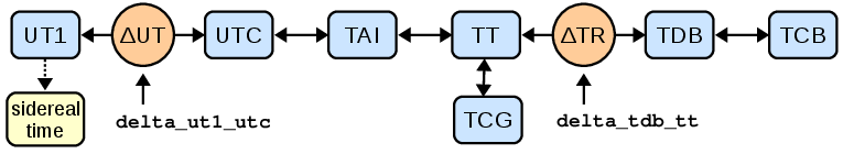
The system of transformation between supported time scales (i.e., all but
local) is shown in the figure below. Further details are provided in the
Convert time scale section.
Scalar or Array#
A Time object can hold either a single time value or an array of time values.
The distinction is made entirely by the form of the input time(s). If a Time
object holds a single value then any format outputs will be a single scalar
value, and likewise for arrays.
Example#
Like other arrays and lists, Time objects holding arrays are subscriptable,
returning scalar or array objects as appropriate:
>>> from astropy.time import Time
>>> t = Time(100.0, format='mjd')
>>> t.jd
np.float64(2400100.5)
>>> t = Time([100.0, 200.0, 300.], format='mjd')
>>> t.jd
array([2400100.5, 2400200.5, 2400300.5])
>>> t[:2]
<Time object: scale='utc' format='mjd' value=[100. 200.]>
>>> t[2]
<Time object: scale='utc' format='mjd' value=300.0>
>>> t = Time(np.arange(50000., 50003.)[:, np.newaxis],
...          np.arange(0., 1., 0.5), format='mjd')
>>> t
<Time object: scale='utc' format='mjd' value=[[50000.  50000.5]
 [50001.  50001.5]
 [50002.  50002.5]]>
>>> t[0]
<Time object: scale='utc' format='mjd' value=[50000.  50000.5]>
NumPy Method Analogs and Applicable NumPy Functions#
For Time instances holding arrays, many of the same methods and attributes
that work on ndarray instances can be used. For example, you can
reshape Time instances and take specific parts using
reshape(), ravel(),
flatten(), T,
transpose(), swapaxes(),
diagonal(), squeeze(), or
take(). Corresponding functions, as well as others
that affect the shape, such as atleast_1d and rollaxis, work
as expected. (The relevant functions have to be explicitly enabled in
astropy source code; let us know if a numpy function is not supported
that you think should work.)
Examples#
To reshape Time instances:
>>> t.reshape(2, 3)
<Time object: scale='utc' format='mjd' value=[[50000.  50000.5 50001. ]
 [50001.5 50002.  50002.5]]>
>>> t.T
<Time object: scale='utc' format='mjd' value=[[50000.  50001.  50002. ]
 [50000.5 50001.5 50002.5]]>
>>> np.roll(t, 1, axis=0)
<Time object: scale='utc' format='mjd' value=[[50002.  50002.5]
 [50000.  50000.5]
 [50001.  50001.5]]>
Note that similarly to the ndarray methods, all but
flatten() try to use new views of the data,
with the data copied only if that is impossible (as discussed, for example, in
the documentation for numpy reshape()).
Some arithmetic methods are supported as well: min(),
max(), ptp(),
sort(), argmin(),
argmax(), and argsort().
To apply arithmetic methods to Time instances:
>>> t.max()
<Time object: scale='utc' format='mjd' value=50002.5>
>>> t.min()
<Time object: scale='utc' format='mjd' value=50000.0>
Inferring Input Format#
The Time class initializer will not accept ambiguous inputs, but it will make
automatic inferences in cases where the inputs are unambiguous. This can apply
when the times are supplied as objects, inputs for ymdhms, or strings. In
the latter case it is not required to specify the format because the available
string formats have no overlap. However, if the format is known in advance the
string parsing will be faster if the format is provided.
Example#
To infer input format:
>>> from datetime import datetime, timezone
>>> t = Time(datetime(2010, 1, 2, 1, 2, 3))
>>> t.format
'datetime'
>>> t = Time('2010-01-02 01:02:03')
>>> t.format
'iso'
Internal Representation#
The Time object maintains an internal representation of time as a pair of
double precision numbers expressing Julian days. The sum of the two numbers is
the Julian Date for that time relative to the given time scale. Users
requiring no better than microsecond precision over human time scales (~100
years) can safely ignore the internal representation details and skip this
section.
This representation is driven by the underlying ERFA C-library implementation.
The ERFA routines take care throughout to maintain overall precision of the
double pair. Users are free to choose the way in which total JD is
provided, though internally one part contains integer days and the
other the fraction of the day, as this ensures optimal accuracy for
all conversions. The internal JD pair is available via the jd1
and jd2 attributes:
>>> t = Time('2010-01-01 00:00:00', scale='utc')
>>> t.jd1, t.jd2
(2455198.0, -0.5)
>>> t2 = t.tai
>>> t2.jd1, t2.jd2
(2455198., -0.49960648148148146)
Creating a Time Object#
The allowed Time arguments to create a time object are listed below:
- valnumpy ndarray, list, str, or number
Data to initialize table.
- val2numpy ndarray, list, str, or number; optional
Data to initialize table.
- formatstr, optional
Format of input value(s).
- scalestr, optional
Time scale of input value(s).
- precisionint between 0 and 9 inclusive
Decimal precision when outputting seconds as floating point.
- in_subfmtstr
Unix glob to select subformats for parsing input times.
- out_subfmtstr
Unix glob to select subformat for output times.
- location
EarthLocationor tuple, optional If a tuple, three
Quantityitems with length units for geocentric coordinates, or a longitude, latitude, and optional height for geodetic coordinates. Can be a single location, or one for each input time.
val#
The val argument specifies the input time or times and can be a single
string or number, or it can be a Python list or numpy array of strings or
numbers. To initialize a Time object based on a specified time, it must be
present.
In most situations, you also need to specify the time scale via the
scale argument. The Time class will never guess the time scale,
so a concise example would be:
>>> t1 = Time(50100.0, scale='tt', format='mjd')
>>> t2 = Time('2010-01-01 00:00:00', scale='utc')
It is possible to create a new Time object from one or more existing time
objects. In this case, the format and scale will be inferred from the
first object unless explicitly specified.
>>> Time([t1, t2])
<Time object: scale='tt' format='mjd' value=[50100. 55197.00076602]>
val2#
The val2 argument is available for those situations where high precision is
required. Recall that the internal representation of time within astropy.time
is two double-precision numbers that when summed give the Julian date. If
provided, the val2 argument is used in combination with val to set the
second of the internal time values. The exact interpretation of val2 is
determined by the input format class. All string-valued formats ignore val2
and all numeric inputs effectively add the two values in a way that maintains
the highest precision. For example:
>>> t = Time(100.0, 0.000001, format='mjd', scale='tt')
>>> t.jd, t.jd1, t.jd2
(np.float64(2400100.500001), 2400101.0, -0.499999)
format#
The format argument sets the time time format, and as mentioned it is
required unless the format can be unambiguously determined from the input times.
scale#
The scale argument sets the time scale and is required except for time
formats such as plot_date (TimePlotDate) and unix
(TimeUnix). These formats represent the duration
in SI seconds since a fixed instant in time is independent of time scale. See
the Time from Epoch Formats for more details.
precision#
The precision setting affects string formats when outputting a value that
includes seconds. It must be an integer between 0 and 9. There is no effect
when inputting time values from strings. The default precision is 3. Note
that the limit of 9 digits is driven by the way that ERFA handles fractional
seconds. In practice this should should not be an issue.
>>> t = Time('B1950.0', precision=3)
>>> t.byear_str
'B1950.000'
>>> t.precision = 0
>>> t.byear_str
'B1950'
in_subfmt#
The in_subfmt argument provides a mechanism to select one or more
subformat values from the available subformats for input. Multiple
allowed subformats can be selected using Unix-style wildcard characters, in
particular * and ?, as documented in the Python fnmatch module.
The default value for in_subfmt is * which matches any available
subformat. This allows for convenient input of values with unknown or
heterogeneous subformat:
>>> Time(['2000:001', '2000:002:03:04', '2001:003:04:05:06.789'])
<Time object: scale='utc' format='yday'
 value=['2000:001:00:00:00.000' '2000:002:03:04:00.000' '2001:003:04:05:06.789']>
You can explicitly specify in_subfmt in order to strictly require a
certain subformat:
>>> t = Time('2000:002:03:04', in_subfmt='date_hm')
>>> t = Time('2000:002', in_subfmt='date_hm')
Traceback (most recent call last):
  ...
ValueError: Input values did not match any of the formats where the
format keyword is optional ['astropy_time', 'datetime',
'byear_str', 'iso', 'isot', 'jyear_str', 'yday']
out_subfmt#
The out_subfmt argument is similar to in_subfmt except that it applies
to output formatting. In the case of multiple matching subformats, the first
matching subformat is used.
>>> Time('2000-01-01 02:03:04', out_subfmt='date').iso
'2000-01-01'
>>> Time('2000-01-01 02:03:04', out_subfmt='date_hms').iso
'2000-01-01 02:03:04.000'
>>> Time('2000-01-01 02:03:04', out_subfmt='date*').iso
'2000-01-01 02:03:04.000'
>>> Time('50814.123456789012345', format='mjd', out_subfmt='str').mjd
'50814.123456789012345'
See also the subformat section.
location#
This optional parameter specifies the observer location, using an
EarthLocation object or a tuple containing any form that can initialize one:
either a tuple with geocentric coordinates (X, Y, Z), or a tuple with geodetic
coordinates (longitude, latitude, height; with height defaulting to zero).
They are used for time scales that are sensitive to observer location
(currently, only TDB, which relies on the PyERFA routine erfa.dtdb to
determine the time offset between TDB and TT), as well as for sidereal time if
no explicit longitude is given.
>>> t = Time('2001-03-22 00:01:44.732327132980', scale='utc',
...          location=('120d', '40d'))
>>> t.sidereal_time('apparent', 'greenwich')
<Longitude 12. hourangle>
>>> t.sidereal_time('apparent')
<Longitude 20. hourangle>
Note
In future versions, we hope to add the possibility to add observatory objects and/or names.
Getting the Current Time#
The current time can be determined as a Time object using the
now class method:
>>> nt = Time.now()
>>> ut = Time(datetime.now(tz=timezone.utc), scale='utc')
The two should be very close to each other.
Fast C-based Date String Parser#
Time formats that are based on a date string representation of time, including
TimeISO, TimeISOT, and
TimeYearDayTime, make use of a fast C-based date parser that
improves speed by a factor of 20 or more for large arrays of times.
The C parser is stricter than the Python-based parser (which relies on
strptime). In particular fields like the month or day of year must
always have a fixed number of ASCII digits. As an example the Python parser will
accept 2000-1-2T3:04:5.23 while the C parser requires
2000-01-02T03:04:05.23
Use of the C parser is enabled by default except when the input subformat
in_subfmt argument is different from the default value of '*'. If the
fast C parser fails to parse the date values then the Time initializer will
automatically fall through to the Python parser.
In rare cases where you need to explicitly control which parser gets used there
is a configuration item time.conf.use_fast_parser that can be set. The
default is 'True', which means to try the fast parser and fall through to
Python parser if needed. Note that the configuration value is a string, not a
bool object.
For example to disable the C parser use:
>>> from astropy.time import conf
>>> date = '2000-1-2T3:04:5.23'
>>> t = Time(date, format='isot')  # Succeeds by default
>>> with conf.set_temp('use_fast_parser', 'False'):
...     t = Time(date, format='isot')
...     print(t)
2000-01-02T03:04:05.230
To force the user of the C parser (for example in testing) use:
>>> with conf.set_temp('use_fast_parser', 'force'):
...     try:
...          t = Time(date, format='isot')
...     except ValueError as err:
...          print(err)
Input values did not match the format class isot:
ValueError: fast C time string parser failed: non-digit found where digit (0-9) required
Using Time Objects#
The operations available with Time objects include:
Get and set time value(s) for an array-valued
Timeobject.Set missing (masked) values.
Get the representation of the time value(s) in a particular time format.
Get a new time object for the same time value(s) but referenced to a different time scale.
Calculate sidereal time and Earth rotation angle corresponding to the time value(s).
Do time arithmetic involving
Time,TimeDeltaand/orQuantityobjects with units of time.
Get and Set Values#
For an existing Time object which is array-valued, you can use the
usual numpy array item syntax to get either a single item or a subset
of items. The returned value is a Time object with all the same
attributes.
Examples#
To get an item or a subset of items:
>>> t = Time(['2001:020', '2001:040', '2001:060', '2001:080'],
...          out_subfmt='date')
>>> print(t[1])
2001:040
>>> print(t[1:])
['2001:040' '2001:060' '2001:080']
>>> print(t[[2, 0]])
['2001:060' '2001:020']
You can also set values in place for an array-valued Time object:
>>> t = Time(['2001:020', '2001:040', '2001:060', '2001:080'],
...          out_subfmt='date')
>>> t[1] = '2010:001'
>>> print(t)
['2001:020' '2010:001' '2001:060' '2001:080']
>>> t[[2, 0]] = '1990:123'
>>> print(t)
['1990:123' '2010:001' '1990:123' '2001:080']
The new value (on the right hand side) when setting can be one of three possibilities:
Scalar string value or array of string values where each value is in a valid time format that can be automatically parsed and used to create a
Timeobject.Value or array of values where each value has the same
formatas theTimeobject being set. For instance, a float ornumpyarray of floats for an object withformat='unix'.Timeobject with identicallocation(butscaleandformatneed not be the same). The right side value will be transformed so the timescalematches.
Whenever any item is set, then the internal cache (see Caching) is cleared
along with the delta_tdb_tt and/or delta_ut1_utc transformation
offsets, if they have been set.
If it is required that the Time object be immutable, then set the
writeable attribute to False. In this case, attempting to set a value will
raise a ValueError: Time object is read-only. See the section on
Caching for an example.
Missing Values#
The Time and TimeDelta objects support functionality for marking values as
missing or invalid. This is also known as masking, and is especially useful for
Table Operations such as joining and stacking.
Example#
You can set one or more items as missing when creating the object in one of two ways. First with a numpy masked array:
>>> dates = np.ma.array(['2001:020', '...', '2001:060'], mask=[False, True, False])
>>> print(Time(dates, out_subfmt="date"))
['2001:020'        ——— '2001:060']
Second with the astropy.utils.masked.Masked class:
>>> from astropy.utils.masked import Masked
>>> dates = Masked(['2001:020', '', '2001:060'], mask=[False, True, False])
>>> t = Time(dates, out_subfmt="date")
>>> print(t)
['2001:020'        ——— '2001:060']
You can also use the special numpy.ma.masked to set a value as missing in an existing
Time object:
>>> t = Time(["2001:020", "2001:040", "2001:060", "2001:080"], out_subfmt="date")
>>> t[2] = np.ma.masked
>>> print(t)
['2001:020' '2001:040'        ——— '2001:080']
If you want to get unmasked data, you can get those either by removing the mask using
the unmasked attribute, or by filling any masked data with a chosen
value:
>>> print(t.unmasked)
['2001:020' '2001:040' '2001:060' '2001:080']
>>> t_filled = t.filled('1999:365')
>>> print(t_filled)
['2001:020' '2001:040' '1999:365' '2001:080']
You can also unset the mask on individual elements by assigning another special value,
numpy.ma.nomask:
>>> t[2] = np.ma.nomask
>>> print(t)
['2001:020' '2001:040' '2001:060' '2001:080']
A subtle difference between the two approaches is that when you unset
the mask by setting with numpy.ma.nomask, a mask is still present
internally, and hence any output will have a mask as well. In
contrast, using unmasked or
filled() removes all masking, and hence any
output is not masked. The masked property can be
used to check whether or not a mask is in use internally:
>>> t.masked
True
>>> t.value
MaskedNDArray(['2001:020', '2001:040', '2001:060', '2001:080'],
            dtype='<U8')
>>> t_filled.masked
False
>>> t_filled.value
array(['2001:020', '2001:040', '1999:365', '2001:080'], dtype='<U8')
Note
When setting the mask, actual time data are kept. However,
when initializing with a masked array, any masked time
input data are overwritten internally, with a time
equivalent to 2000-01-01 12:00:00 (in the same scale and
format as the other values). This is to ensure no errors or
warnings are raised by invalid data hidden by the mask.
Hence, for initialization with masked data, there is no way
to recover the original masked values:
>>> dates = Masked(['2001:020', '2001:040', '2001:060'],
...                mask=[False, True, False])
>>> tm = Time(dates, out_subfmt="date")
>>> tm[2] = np.ma.masked
>>> print(tm)
['2001:020'        ———        ———]
>>> print(tm.unmasked)
['2001:020' '2000:001' '2001:060']
Once one or more values in the object are masked, any operations will
propagate those values as masked, and access to format attributes such
as unix or value will return a Masked object:
>>> t[1:3] = np.ma.masked
>>> t.isot
MaskedNDArray(['2001-01-20',          ———,          ———, '2001-03-21'],
              dtype='<U10')
You can view the mask, but note that it is read-only. Setting and
clearing the mask is always done by setting the item to
masked and nomask, respectively.
>>> t.mask
array([False, True,  True, False])
Choice of Masked Array Type#
Time internally uses astropy’s Masked class to represent the mask. It is
possible to initialize with data using numpy’s MaskedArray class,
but by default all output will use Masked. For backward compatibility, it is
possible to set masked_array_type to “numpy” to ensure
that output uses MaskedArray where possible (for all but Quantity).
Custom Format Classes and Masked Values#
For advanced users who have written a custom time format via a
TimeFormat subclass, it may be necessary to modify your class
if you wish to support masked values, and especially if you earlier
supported having missing values by setting the jd2 attribute to
numpy.nan. For applications that do not need masked or missing values, no
changes are required.
Prior to astropy 6.0, missing values in a TimeFormat subclass
object were marked by setting the corresponding entries of the jd2
attribute to be numpy.nan (but this was never done directly by the user).
Since astropy 6.0, instead Masked arrays are used, and these are written to
propagate properly through (almost) all numpy and ERFA functions.
In general, very few modifications should be needed to support Masked
arrays. Generally, on input, no changes are needed since the format will be
given unmasked values (with any masked input values replaced with the default
value to ensure that only valid values are passed in). Some care may
need to be taken, though, that the mask is propagated properly in calculating
output values from jd1 to jd2 in the value property.
Get Representation#
Instants of time can be represented in different ways, for instance as an
ISO-format date string ('1999-07-23 04:31:00') or seconds since 1998.0
(49091460.0) or Modified Julian Date (51382.187451574).
The representation of a Time object in a particular format is available
by getting the object attribute corresponding to the format name. The list of
available format names is in the time format section.
>>> t = Time('2010-01-01 00:00:00', format='iso', scale='utc')
>>> t.jd        # JD representation of time in current scale (UTC)
np.float64(2455197.5)
>>> t.iso       # ISO representation of time in current scale (UTC)
'2010-01-01 00:00:00.000'
>>> t.unix      # seconds since 1970.0 (UTC)
np.float64(1262304000.0)
>>> t.datetime  # Representation as datetime.datetime object
datetime.datetime(2010, 1, 1, 0, 0)
Example#
To get the representation of a Time object:
>>> import matplotlib.pyplot as plt
>>> jyear = np.linspace(2000, 2001, 20)
>>> t = Time(jyear, format='jyear')
>>> fig, ax = plt.subplots()
>>> ax.scatter(t.datetime, jyear)
>>> fig.autofmt_xdate()  # orient date labels at a slant
>>> fig.show()
Convert Time Scale#
A new Time object for the same time value(s) but referenced to a new time
scale can be created getting the object attribute corresponding to the time
scale name. The list of available time scale names is in the time scale
section and in the figure below illustrating the network of time scale
transformations.
Examples#
To create a Time object with a new time scale:
>>> t = Time('2010-01-01 00:00:00', format='iso', scale='utc')
>>> t.tt        # TT scale
<Time object: scale='tt' format='iso' value=2010-01-01 00:01:06.184>
>>> t.tai
<Time object: scale='tai' format='iso' value=2010-01-01 00:00:34.000>
In this process the format and other object attributes like lon,
lat, and precision are also propagated to the new object.
As noted in the Time Object Basics section, a Time object can only be
changed by explicitly setting some of its elements. The process of changing the
time scale therefore begins by making a copy of the original object and then
converting the internal time values in the copy to the new time scale. The new
Time object is returned by the attribute access.
Caching#
The computations for transforming to different time scales or formats can be
time-consuming for large arrays. In order to avoid repeated computations, each
Time or TimeDelta instance caches such transformations internally:
>>> t = Time(np.arange(1e6), format='unix', scale='utc')

>>> time x = t.tt
CPU times: user 263 ms, sys: 4.02 ms, total: 267 ms
Wall time: 267 ms

>>> time x = t.tt
CPU times: user 28 µs, sys: 9 µs, total: 37 µs
Wall time: 32.9 µs
Actions such as changing the output precision or subformat will clear the cache. In order to explicitly clear the internal cache do:
>>> del t.cache

>>> time x = t.tt
CPU times: user 263 ms, sys: 4.02 ms, total: 267 ms
Wall time: 267 ms
In order to ensure consistency between the transformed (and cached) version and the original, the transformed object is set to be not writeable. For example:
>>> x = t.tt
>>> x[1] = '2000:001'
Traceback (most recent call last):
  ...
ValueError: Time object is read-only. Make a copy() or set "writeable" attribute to True.
If you require modifying the object then make a copy first, for example, x =
t.tt.copy().
Transformation Offsets#
Time scale transformations that cross one of the orange circles in the image above require an additional offset time value that is model or observation dependent. See SOFA Time Scale and Calendar Tools for further details.
The two attributes delta_ut1_utc and
delta_tdb_tt provide a way to set
these offset times explicitly. These represent the time scale offsets
UT1 - UTC and TDB - TT, respectively. As an example:
>>> t = Time('2010-01-01 00:00:00', format='iso', scale='utc')
>>> t.delta_ut1_utc = 0.334  # Explicitly set one part of the transformation
>>> t.ut1.iso    # ISO representation of time in UT1 scale
'2010-01-01 00:00:00.334'
For the UT1 to UTC offset, you have to interpolate the observed values provided
by the International Earth Rotation and Reference Systems (IERS) Service. astropy will automatically download and use values
from the IERS which cover times spanning from 1973-Jan-01 through one year into
the future. In addition, the astropy package is bundled with a data table of
values provided in Bulletin B, which cover the period from 1962 to shortly
before an astropy release.
When the delta_ut1_utc attribute is not set
explicitly, IERS values will be used (initiating a download of a few Mb
file the first time). For details about how IERS values are used in astropy
time and coordinates, and to understand how to control automatic downloads, see
IERS data access (astropy.utils.iers). The example below illustrates converting to the UT1
scale along with the auto-download feature:
>>> t = Time('2016:001')
>>> t.ut1
Downloading https://maia.usno.navy.mil/ser7/finals2000A.all
|==================================================================| 3.0M/3.0M (100.00%)         6s
<Time object: scale='ut1' format='yday' value=2016:001:00:00:00.082>
Note
The IERS_Auto class contains machinery
to ensure that the IERS table is kept up to date by auto-downloading the
latest version as needed. This means that the IERS table is assured of
having the state-of-the-art definitive and predictive values for Earth
rotation. As a user it is your responsibility to understand the
accuracy of IERS predictions if your science depends on that. If you
request UT1-UTC for times beyond the range of IERS table data then the
nearest available values will be provided.
In the case of the TDB to TT offset, most users need only provide the
location when creating the Time object. If the
delta_tdb_tt attribute is not explicitly set, then
the PyERFA routine erfa.dtdb will be used to compute the TDB to TT
offset. If location is not specified, the center of the Earth is assumed.
Example#
The following code replicates an example in the SOFA Time Scale and Calendar Tools document. It does the transform from UTC to all supported time scales (TAI, TCB, TCG, TDB, TT, UT1, UTC). This requires an observer location (here, latitude and longitude).
>>> import astropy.units as u
>>> t = Time('2006-01-15 21:24:37.5', format='iso', scale='utc',
...          location=(-155.933222*u.deg, 19.48125*u.deg))
>>> t.utc.iso
'2006-01-15 21:24:37.500'
>>> t.ut1.iso
'2006-01-15 21:24:37.834'
>>> t.tai.iso
'2006-01-15 21:25:10.500'
>>> t.tt.iso
'2006-01-15 21:25:42.684'
>>> t.tcg.iso
'2006-01-15 21:25:43.323'
>>> t.tdb.iso
'2006-01-15 21:25:42.684'
>>> t.tcb.iso
'2006-01-15 21:25:56.894'
Hashing#
A user can generate a unique hash key for scalar (0-dimensional) Time or
TimeDelta objects. The key is based on a tuple of jd1,
jd2, scale, and location (if present, None otherwise).
Note that two Time objects with a different scale can compare equally
but still have different hash keys. This a practical consideration driven
in by performance, but in most cases represents a desirable behavior.
Printing Time Arrays#
If your times array contains a lot of elements, the value argument will
display all the elements of the Time object t when it is called or
printed. To control the number of elements to be displayed, set the
threshold argument with np.printoptions as follows:
>>> many_times = np.arange(1000)
>>> t = Time(many_times, format='cxcsec')
>>> with np.printoptions(threshold=10):
...     print(repr(t))
...     print(t.iso)
<Time object: scale='tt' format='cxcsec' value=[  0.   1.   2. ... 997. 998. 999.]>
['1998-01-01 00:00:00.000' '1998-01-01 00:00:01.000'
 '1998-01-01 00:00:02.000' ... '1998-01-01 00:16:37.000'
 '1998-01-01 00:16:38.000' '1998-01-01 00:16:39.000']
Sidereal Time and Earth Rotation Angle#
Apparent or mean sidereal time can be calculated using
sidereal_time(). The method returns a Longitude
with units of hour angle, which by default is for the longitude corresponding to
the location with which the Time object is initialized. Like the scale
transformations, ERFA C-library routines are used under the hood, which support
calculations following different IAU resolutions.
Similarly, one can calculate the Earth rotation angle with
earth_rotation_angle(). Unlike sidereal time, which
is referred to the equinox and is a complicated function of both UT1 and
Terrestrial Time, the Earth rotation angle is referred to the Celestial
Intermediate Origin (CIO) and is a linear function of UT1 alone.
For the recent IAU precession models, as well as for the Earth rotation angle, the result includes the TIO locator (s’), which positions the Terrestrial Intermediate Origin on the equator of the Celestial Intermediate Pole (CIP) and is rigorously corrected for polar motion.
Example#
To calculate sidereal time:
>>> t = Time('2006-01-15 21:24:37.5', scale='utc', location=('120d', '45d'))
>>> t.sidereal_time('mean')
<Longitude 13.08952187 hourangle>
>>> t.sidereal_time('apparent')
<Longitude 13.08950368 hourangle>
>>> t.earth_rotation_angle()
<Longitude 13.08436206 hourangle>
>>> t.sidereal_time('apparent', 'greenwich')
<Longitude 5.08950368 hourangle>
>>> t.sidereal_time('apparent', '-90d')
<Longitude 23.08950368 hourangle>
>>> t.sidereal_time('apparent', '-90d', 'IAU1994')
<Longitude 23.08950365 hourangle>
Time Deltas#
Time arithmetic is supported using the TimeDelta class. The following
operations are available:
Create a
TimeDeltaexplicitly by instantiating a class object.Negate a
TimeDeltaor take its absolute value.Multiply or divide a
TimeDeltaby a constant or array.
The TimeDelta class is derived from the Time class and shares many of its
properties. One difference is that the time scale has to be one for which one
day is exactly 86400 seconds. Hence, the scale cannot be UTC.
Quantity objects with time units can also be used in place of TimeDelta.
The available time formats are:
Format |
Class |
|---|---|
sec |
|
jd |
|
datetime |
|
quantity_str |
Examples#
Use of the TimeDelta object is illustrated in the few examples below:
>>> t1 = Time('2010-01-01 00:00:00')
>>> t2 = Time('2010-02-01 00:00:00')
>>> dt = t2 - t1  # Difference between two Times
>>> dt
<TimeDelta object: scale='tai' format='jd' value=31.0>
>>> dt.sec
np.float64(2678400.0)

>>> from astropy.time import TimeDelta
>>> dt2 = TimeDelta(50.0, format='sec')
>>> t3 = t2 + dt2  # Add a TimeDelta to a Time
>>> t3.iso
'2010-02-01 00:00:50.000'

>>> t2 - dt2  # Subtract a TimeDelta from a Time
<Time object: scale='utc' format='iso' value=2010-01-31 23:59:10.000>

>>> dt + dt2
<TimeDelta object: scale='tai' format='jd' value=31.0005787037>

>>> import numpy as np
>>> t1 + dt * np.linspace(0, 1, 5)
<Time object: scale='utc' format='iso' value=['2010-01-01 00:00:00.000'
'2010-01-08 18:00:00.000' '2010-01-16 12:00:00.000' '2010-01-24 06:00:00.000'
'2010-02-01 00:00:00.000']>

>>> import astropy.units as u
>>> t1 + 1 * u.hour
<Time object: scale='utc' format='iso' value=2010-01-01 01:00:00.000>
A human-readable multi-scale format for string representation of a time delta is
available via the quantity_str format. See the
TimeDeltaQuantityString class docstring for more details:
>>> TimeDelta(40.1 * u.hr).quantity_str
'1d 16hr 6min'
>>> t4 = TimeDelta("-1yr 2d 23hr 10min 5.6s")
>>> print(t4)
-368d 5hr 10min 5.6s
>>> t4.to_value(subfmt="d")
'-368.215d'
The now deprecated default assumes days for numeric inputs:
>>> t1 + 5.0
<Time object: scale='utc' format='iso' value=2010-01-06 00:00:00.000>
TimeDeltaMissingUnitWarning: Numerical value without unit or explicit format passed to TimeDelta, assuming days
The TimeDelta has a to_value method which supports
controlling the type of the output representation by providing either a format
name and optional subformat or a valid astropy unit:
>>> dt.to_value(u.hr)
np.float64(744.0)
>>> dt.to_value('jd', 'str')
'31.0'
Time Scales for Time Deltas#
We have shown in the above that the difference between two UTC times is a
TimeDelta with a scale of TAI. This is because a UTC time difference cannot be
uniquely defined unless the user knows the two times that were differenced
(because of leap seconds, a day does not always have 86400 seconds). For all
other time scales, the TimeDelta inherits the scale of the first Time
object.
Examples#
To get the time scale for a TimeDelta object:
>>> t1 = Time('2010-01-01 00:00:00', scale='tcg')
>>> t2 = Time('2011-01-01 00:00:00', scale='tcg')
>>> dt = t2 - t1
>>> dt
<TimeDelta object: scale='tcg' format='jd' value=365.0>
When TimeDelta objects are added or subtracted from Time objects, scales
are converted appropriately, with the final scale being that of the Time
object:
>>> t2 + dt
<Time object: scale='tcg' format='iso' value=2012-01-01 00:00:00.000>
>>> t2.tai
<Time object: scale='tai' format='iso' value=2010-12-31 23:59:27.068>
>>> t2.tai + dt
<Time object: scale='tai' format='iso' value=2011-12-31 23:59:27.046>
TimeDelta objects can be converted only to objects with compatible scales
(i.e., scales for which it is not necessary to know the times that were
differenced):
>>> dt.tt
<TimeDelta object: scale='tt' format='jd' value=364.999999746>
>>> dt.tdb
Traceback (most recent call last):
  ...
ScaleValueError: Cannot convert TimeDelta with scale 'tcg' to scale 'tdb'
TimeDelta objects can also have an undefined scale, in which case it is
assumed that their scale matches that of the other Time or TimeDelta
object (or is TAI in case of a UTC time):
>>> t2.tai + TimeDelta(365., format='jd', scale=None)
<Time object: scale='tai' format='iso' value=2011-12-31 23:59:27.068>
Note
Since internally Time uses floating point numbers, round-off
errors can cause two times to be not strictly equal even if
mathematically they should be. For times in UTC in particular, this
can lead to surprising behavior, because when you add a
TimeDelta, which cannot have a scale of UTC, the UTC time is
first converted to TAI, then the addition is done, and finally the
time is converted back to UTC. Hence, rounding errors can be
incurred, which means that even expected equalities may not hold:
>>> t = Time(2450000., 1e-6, format='jd')
>>> t + TimeDelta(0, format='jd') == t
False
Barycentric and Heliocentric Light Travel Time Corrections#
The arrival times of photons at an observatory are not particularly useful for accurate timing work, such as eclipse/transit timing of binaries or exoplanets. This is because the changing location of the observatory causes photons to arrive early or late. The solution is to calculate the time the photon would have arrived at a standard location; either the Solar System barycenter or the heliocenter.
Example#
Suppose you observed the dwarf nova IP Peg from Greenwich and have a list of
times in MJD form, in the UTC timescale. You then create appropriate Time and
SkyCoord objects and calculate light travel times to the barycenter as
follows:
>>> from astropy import time, coordinates as coord, units as u
>>> ip_peg = coord.SkyCoord("23:23:08.55", "+18:24:59.3",
...                         unit=(u.hourangle, u.deg), frame='icrs')
>>> greenwich = coord.EarthLocation.of_site('greenwich')
>>> times = time.Time([56325.95833333, 56325.978254], format='mjd',
...                   scale='utc', location=greenwich)
>>> ltt_bary = times.light_travel_time(ip_peg)
>>> ltt_bary
<TimeDelta object: scale='tdb' format='jd' value=[-0.0037715  -0.00377286]>
If you desire the light travel time to the heliocenter instead, then use:
>>> ltt_helio = times.light_travel_time(ip_peg, 'heliocentric')
>>> ltt_helio
<TimeDelta object: scale='tdb' format='jd' value=[-0.00376576 -0.00376712]>
The method returns an TimeDelta object, which can be added to
your times to give the arrival time of the photons at the barycenter or
heliocenter. Here, you should be careful with the timescales used; for more
detailed information about timescales, see Time Scale.
The heliocenter is not a fixed point, and therefore the gravity continually changes at the heliocenter. Thus, the use of a relativistic timescale like TDB is not particularly appropriate, and, historically, times corrected to the heliocenter are given in the UTC timescale:
>>> times_heliocentre = times.utc + ltt_helio
Corrections to the barycenter are more precise than the heliocenter, because the barycenter is a fixed point where gravity is constant. For maximum accuracy you want to have your barycentric corrected times in a timescale that has always ticked at a uniform rate, and ideally one whose tick rate is related to the rate that a clock would tick at the barycenter. For this reason, barycentric corrected times normally use the TDB timescale:
>>> time_barycentre = times.tdb + ltt_bary
By default, the light travel time is calculated using the position and velocity of Earth and the Sun from ERFA routines, but you can also get more precise calculations using the JPL ephemerides (which are derived from dynamical models). An example using the JPL ephemerides is:
>>> ltt_bary_jpl = times.light_travel_time(ip_peg, ephemeris='jpl')
>>> ltt_bary_jpl
<TimeDelta object: scale='tdb' format='jd' value=[-0.0037715  -0.00377286]>
>>> (ltt_bary_jpl - ltt_bary).to(u.ms)
<Quantity [-0.00132325, -0.00132861] ms>
The difference between the built-in ephemerides and the JPL ephemerides is normally of the order of 1/100th of a millisecond, so the built-in ephemerides should be suitable for most purposes. For more details about what ephemerides are available, including the requirements for using JPL ephemerides, see Solar System Ephemerides.
Interaction with time-like Quantities#
Where possible, Quantity objects with units of time are treated as TimeDelta
objects with undefined scale (though necessarily with lower precision). They
can also be used as input in constructing Time and TimeDelta objects, and
TimeDelta objects can be converted to Quantity objects of arbitrary units
of time.
Examples#
To use Quantity objects with units of time:
>>> import astropy.units as u
>>> Time(10.*u.yr, format='gps')   # time-valued quantities can be used for
...                                # for formats requiring a time offset
<Time object: scale='tai' format='gps' value=315576000.0>
>>> Time(10.*u.yr, 1.*u.s, format='gps')
<Time object: scale='tai' format='gps' value=315576001.0>
>>> Time(2000.*u.yr, format='jyear')
<Time object: scale='tt' format='jyear' value=2000.0>
>>> Time(2000.*u.yr, format='byear')
...                                # but not for Besselian year, which implies
...                                # a different time scale
...
Traceback (most recent call last):
  ...
ValueError: Input values did not match the format class byear:
ValueError: cannot use Quantities for 'byear' format, as the unit of year is defined as 365.25 days, while the length of year is variable in this format. Use float instead.

>>> TimeDelta(10.*u.yr)            # With a quantity, no format is required
<TimeDelta object: scale='None' format='jd' value=3652.5>

>>> dt = TimeDelta([10., 20., 30.], format='jd')
>>> dt.to(u.hr)                    # can convert TimeDelta to a quantity
<Quantity [240., 480., 720.] h>
>>> dt > 400. * u.hr               # and compare to quantities with units of time
array([False,  True,  True]...)
>>> dt + 1.*u.hr                   # can also add/subtract such quantities
<TimeDelta object: scale='None' format='jd' value=[10.04166667 20.04166667 30.04166667]>
>>> Time(50000., format='mjd', scale='utc') + 1.*u.hr
<Time object: scale='utc' format='mjd' value=50000.0416667>
>>> dt * 10.*u.km/u.s              # for multiplication and division with a
...                                # Quantity, TimeDelta is converted
<Quantity [100., 200., 300.] d km / s>
>>> dt * 10.*u.Unit(1)             # unless the Quantity is dimensionless
<TimeDelta object: scale='None' format='jd' value=[100. 200. 300.]>
Writing a Custom Format#
Some applications may need a custom Time format, and this capability is
available by making a new subclass of the TimeFormat class.
When such a subclass is defined in your code, the format class and
corresponding name is automatically registered in the set of available time
formats.
Examples#
The key elements of a new format class are illustrated by examining the
code for the jd format (which is one of the most minimal):
class TimeJD(TimeFormat):
    """
    Julian Date time format.
    """
    name = 'jd'  # Unique format name

    def set_jds(self, val1, val2):
        """
        Set the internal jd1 and jd2 values from the input val1, val2.
        The input values are expected to conform to this format, as
        validated by self._check_val_type(val1, val2) during __init__.
        """
        self._check_scale(self._scale)  # Validate scale.
        self.jd1, self.jd2 = day_frac(val1, val2)

    @property
    def value(self):
        """
        Return format ``value`` property from internal jd1, jd2
        """
        return self.jd1 + self.jd2
As mentioned above, the _check_val_type(self, val1, val2)
method may need to be overridden to validate the inputs as conforming to the
format specification. By default this checks for valid float, float array, or
Quantity inputs. In contrast, the iso format class ensures the inputs
meet the ISO format specification for strings.
One special case that is relatively common and more convenient to implement is a
format that makes a small change to the date format. For instance, you could
insert T in the yday format with the following TimeYearDayTimeCustom
class. Notice how the subfmts definition is modified slightly from the
standard TimeISO class from which it inherits:
>>> from astropy.time import TimeISO
>>> class TimeYearDayTimeCustom(TimeISO):
...    """
...    Year, day-of-year and time as "<YYYY>-<DOY>T<HH>:<MM>:<SS.sss...>".
...    The day-of-year (DOY) goes from 001 to 365 (366 in leap years).
...    For example, 2000-001T00:00:00.000 is midnight on January 1, 2000.
...    The allowed subformats are:
...    - 'date_hms': date + hours, mins, secs (and optional fractional secs)
...    - 'date_hm': date + hours, mins
...    - 'date': date
...    """
...    name = 'yday_custom'  # Unique format name
...    subfmts = (('date_hms',
...                '%Y-%jT%H:%M:%S',
...                '{year:d}-{yday:03d}T{hour:02d}:{min:02d}:{sec:02d}'),
...               ('date_hm',
...                '%Y-%jT%H:%M',
...                '{year:d}-{yday:03d}T{hour:02d}:{min:02d}'),
...               ('date',
...                '%Y-%j',
...                '{year:d}-{yday:03d}'))


>>> t = Time('2000-01-01')
>>> t.yday_custom
'2000-001T00:00:00.000'
>>> t2 = Time('2016-001T00:00:00')
>>> t2.iso
'2016-01-01 00:00:00.000'
Another special case that is relatively common is a format that represents the
time since a particular epoch. The classic example is Unix time which is the
number of seconds since 1970-01-01 00:00:00 UTC, not counting leap seconds. What
if we wanted that value but do want to count leap seconds. This would be
done by using the TAI scale instead of the UTC scale. In this case we inherit
from the TimeFromEpoch class and define a few class attributes:
>>> from astropy.time.formats import erfa, TimeFromEpoch
>>> class TimeUnixLeap(TimeFromEpoch):
...    """
...    Seconds from 1970-01-01 00:00:00 TAI.  Similar to Unix time
...    but this includes leap seconds.
...    """
...    name = 'unix_leap'
...    unit = 1.0 / erfa.DAYSEC  # in days (1 day == 86400 seconds)
...    epoch_val = '1970-01-01 00:00:00'
...    epoch_val2 = None
...    epoch_scale = 'tai'  # Scale for epoch_val class attribute
...    epoch_format = 'iso'  # Format for epoch_val class attribute

>>> t = Time('2000-01-01')
>>> t.unix_leap
np.float64(946684832.0)
>>> t.unix_leap - t.unix
np.float64(32.0)
Going beyond this will probably require looking at the astropy code for more
guidance, but if you get stuck, the astropy developers are more than happy
to help. If you write a format class that is widely useful we might want to
include it in the core!
Timezones#
When a Time object is constructed from a timezone-aware
datetime, no timezone information is saved in the
Time object. However, Time objects can be
converted to timezone-aware datetime objects.
Example#
To convert a Time object to a timezone-aware datetime object:
>>> from datetime import datetime
>>> from astropy.time import Time, TimezoneInfo
>>> import astropy.units as u
>>> utc_plus_one_hour = TimezoneInfo(utc_offset=1*u.hour)
>>> dt_aware = datetime(2000, 1, 1, 0, 0, 0, tzinfo=utc_plus_one_hour)
>>> t = Time(dt_aware)  # Loses timezone info, converts to UTC
>>> print(t)            # will return UTC
1999-12-31 23:00:00
>>> print(t.to_datetime(timezone=utc_plus_one_hour)) # to timezone-aware datetime
2000-01-01 00:00:00+01:00
Timezone database packages, like pytz
for example, may be more convenient to use to create tzinfo
objects used to specify timezones rather than the TimezoneInfo
object.
Example#
Using the dateutil package,
you can parse times in a wide variety of supported formats to generate a
datetime.datetime object which can then be used to initialize a Time object:
>>> from dateutil.parser import parse
>>> dtime = parse('2020-10-29T08:20:46.950+1100')
>>> Time(dtime)
<Time object: scale='utc' format='datetime' value=2020-10-28 21:20:46.950000>
Custom String Formats with strftime and strptime#
The Time object supports output string representation
using the format specification language defined in the Python standard library
for time.strftime. This can be done using the strftime
method.
Examples#
To get output string representation using the strftime
method:
>>> from astropy.time import Time
>>> t = Time('2018-01-01T10:12:58')
>>> t.strftime('%H:%M:%S %d %b %Y')
'10:12:58 01 Jan 2018'
Conversely, to create a Time object from a custom date string
that can be parsed with Python standard library time.strptime (using the same
format language linked above), use the strptime class
method:
>>> from astropy.time import Time
>>> t = Time.strptime('23:59:60 30 June 2015', '%H:%M:%S %d %B %Y')
>>> t
<Time object: scale='utc' format='isot' value=2015-06-30T23:59:60.000>
Performance Tips#
Here we provide some tips and tricks for how to optimize performance of code
using astropy.time.
Broadcasting#
Like most of Astropy’s classes, Time can be array-valued and fully
supports NumPy’s broadcasting rules.
The best performance will generally be had when making full use of that.
For instance, when one wants to calculate the light travel time for
a large number of sources, rather than loop over them, it is substantially
faster to put all the sources inside a single SkyCoord instance and
pass that to light_travel_time(). For a detailed
example, see Determining and plotting the altitude/azimuth of a celestial object.
Reference/API#
Acknowledgments and Licenses#
This package makes use of the PyERFA wrappers of the ERFA ANSI C library. The copyright of the ERFA software belongs to the NumFOCUS Foundation. The library is made available under the terms of the “BSD-three clauses” license.
The ERFA library is derived, with permission, from the International Astronomical Union’s “Standards of Fundamental Astronomy” (SOFA) library, available from https://www.iausofa.org.