JointFitter#
There are cases where one may wish to fit multiple datasets with models that
share parameters. This is possible with the
astropy.modeling.fitting.JointFitter. Basically, this fitter is
setup with a list of defined models, the parameters in common between the
different models, and the initial values for those parameters. Then the fitter
is called supplying as many x and y arrays, one for each model to be fit. The
fit parameters are the result of the jointly fitting the models to the
combined datasets.
Note
The JointFitter uses the scipy.optimize.leastsq. In addition, it does not support fixed, bounded, or tied parameters at this time.
Example: Spectral Line#
This example is for two spectral segments with different spectral resolutions that have the same spectral line in the wavelength region that is overlapping between both segments.
We will need to define a Gaussian function that has mean wavelength, area, and
width parameters. This is needed as the astropy.modeling.functional_models.Gaussian1D
function has mean wavelength, central intensity, and width parameters, but the
central intensity of a line will be different at different spectral resolutions,
but the area will be the same.
First, imports needed for this example
>>> # imports
>>> import math
>>> import numpy as np
>>> from astropy.modeling import fitting, Fittable1DModel
>>> from astropy.modeling.parameters import Parameter
>>> from astropy.modeling.functional_models import FLOAT_EPSILON
Now define AreaGaussian1D with area instead of intensity as a parameter. This new is modified and trimmed version of the standard Gaussian1D model.
>>> class AreaGaussian1D(Fittable1DModel):
...   """
...   One dimensional Gaussian model with area as a parameter.
...
...   Parameters
...   ----------
...   area : float or `~astropy.units.Quantity`.
...       Integrated area
...       Note: amplitude = area / (stddev * np.sqrt(2 * np.pi))
...   mean : float or `~astropy.units.Quantity`.
...       Mean of the Gaussian.
...   stddev : float or `~astropy.units.Quantity`.
...       Standard deviation of the Gaussian with FWHM = 2 * stddev * np.sqrt(2 * np.log(2)).
...   """
...   area = Parameter(default=1)
...   mean = Parameter(default=0)
...
...   # Ensure stddev makes sense if its bounds are not explicitly set.
...   # stddev must be non-zero and positive.
...   stddev = Parameter(default=1, bounds=(FLOAT_EPSILON, None))
...
...   @staticmethod
...   def evaluate(x, area, mean, stddev):
...       """
...       AreaGaussian1D model function.
...       """
...       return (area / (stddev * np.sqrt(2 * np.pi))) * np.exp(
...           -0.5 * (x - mean) ** 2 / stddev ** 2
...       )
Data to be fit is simulated. The 1st spectral segment will have a spectral resolution that is a factor of 2 higher than the second segment. The first segment will have wavelengths from 1 to 6 and the second from 4 to 10 giving an overlapping wavelength region from 4 to 6.
>>> # Generate fake data
>>> mean = 5.1
>>> sigma1 = 0.2
>>> sigma2 = 0.4
>>> noise = 0.10
>>> # compute the central amplitudes so the lines in each segment have the
>>> # same area
>>> area = 1.5
>>> amp1 = area / np.sqrt(2.0 * math.pi * sigma1 ** 2)
>>> amp2 = area / np.sqrt(2.0 * math.pi * sigma2 ** 2)
>>> # segment 1
>>> rng = np.random.default_rng(147)
>>> x1 = np.linspace(1.0, 6.0, 200)
>>> y1 = amp1 * np.exp(-0.5 * (x1 - mean) ** 2 / sigma1 ** 2)
>>> y1 += rng.normal(0.0, noise, x1.shape)
>>> # segment 2
>>> x2 = np.linspace(4.0, 10.0, 200)
>>> y2 = amp2 * np.exp(-0.5 * (x2 - mean) ** 2 / sigma2 ** 2)
>>> y2 += rng.normal(0.0, noise, x2.shape)
Now define the models to be fit and fitter to use. Then fit the two simulated datasets.
>>> # define the two models to be fit
>>> gjf1 = AreaGaussian1D(area=1.0, mean=5.0, stddev=1.0)
>>> gjf2 = AreaGaussian1D(area=1.0, mean=5.0, stddev=1.0)
>>> # define the jointfitter specifying the parameters in common and their initial values
>>> fit_joint = fitting.JointFitter(
...    [gjf1, gjf2], {gjf1: ["area", "mean"], gjf2: ["area", "mean"]}, [1.0, 5.0]
... )
>>>
>>> # perform the fit
>>> g12 = fit_joint(x1, y1, x2, y2)
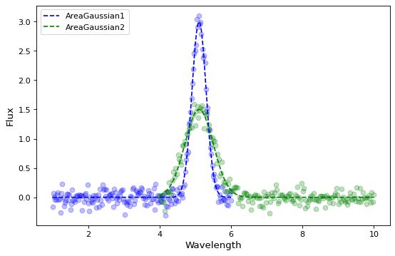
The resulting fit parameters show that the area and mean wavelength of the two AreaGaussian1D models are exactly the same while the width (stddev) is different reflecting the different spectral resolutions of the two segments.
AreaGaussian1 parameters
>>> print(gjf1.param_names)
('area', 'mean', 'stddev')
>>> print(gjf1.parameters)
[1.49823951 5.10494811 0.19918164]
AreaGaussian2 parameters
>>> print(gjf1.param_names)
('area', 'mean', 'stddev')
>>> print(gjf2.parameters)
[1.49823951 5.10494811 0.39860539]
The simulated data and best fit models can be plotted showing good agreement between the two AreaGaussian1D models and the two spectral segments.