Physical Models#
These are models that are physical motivated, generally as solutions to physical problems. This is in contrast to those that are mathematically motivated, generally as solutions to mathematical problems.
BlackBody#
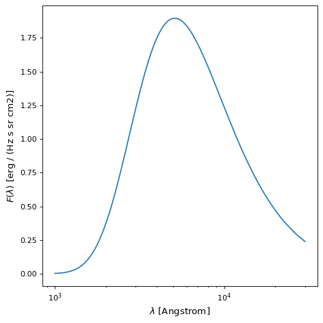
The BlackBody model provides a model
for using Planck’s Law.
The blackbody function is
where \(\nu\) is the frequency, \(T\) is the temperature, \(A\) is the scaling factor, \(h\) is the Plank constant, \(c\) is the speed of light, and \(k\) is the Boltzmann constant.
The two parameters of the model the scaling factor scale (A) and
the absolute temperature temperature (T). If the scale factor does not
have units, then the result is in units of spectral radiance, specifically
ergs/(cm^2 Hz s sr). If the scale factor is passed with spectral radiance units,
then the result is in those units (e.g., ergs/(cm^2 A s sr) or MJy/sr).
Setting the scale factor with units of ergs/(cm^2 A s sr) will give the
Planck function as \(B_\lambda\).
The temperature can be passed as a Quantity with any supported temperature unit.
An example plot for a blackbody with a temperature of 10000 K and a scale of 1 is
shown below. A scale of 1 shows the Planck function with no scaling in the
default units returned by BlackBody.
import numpy as np
import matplotlib.pyplot as plt

from astropy.modeling.models import BlackBody
import astropy.units as u

wavelengths = np.logspace(np.log10(1000), np.log10(3e4), num=1000) * u.AA

# blackbody parameters
temperature = 10000 * u.K

# BlackBody provides the results in ergs/(cm^2 Hz s sr) when scale has no units
bb = BlackBody(temperature=temperature, scale=10000.0)
bb_result = bb(wavelengths)

fig, ax = plt.subplots(layout='tight')
ax.plot(wavelengths, bb_result, '-')

ax.set(
    xscale="log",
    xlabel=fr"$\lambda$ [{wavelengths.unit}]",
    ylabel=fr"$F(\lambda)$ [{bb_result.unit}]",
)

plt.show()
The bolometric_flux() member
function gives the bolometric flux using
\(\sigma T^4/\pi\) where \(\sigma\) is the Stefan-Boltzmann constant.
The lambda_max() and
nu_max() member functions
give the wavelength and frequency of the maximum for \(B_\lambda\)
and \(B_\nu\), respectively, calculated using Wien’s Law.
Drude1D#
The Drude1D model provides a model
for the behavior of an electron in a material
(see Drude Model).
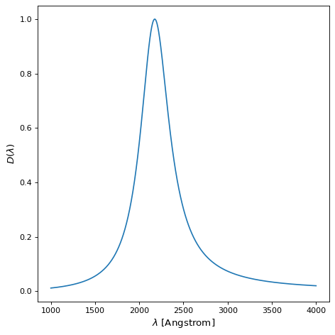
Like the Lorentz1D model, the Drude model
has broader wings than the Gaussian1D
model. The Drude profile has been used to model dust features including the
2175 Angstrom extinction feature and the mid-infrared aromatic/PAH features.
The Drude function at \(x\) is
where \(A\) is the amplitude, \(f\) is the full width at half maximum, and \(x_0\) is the central wavelength. An example of a Drude1D model with \(x_0 = 2175\) Angstrom and \(f = 400\) Angstrom is shown below.
import numpy as np
import matplotlib.pyplot as plt

from astropy.modeling.models import Drude1D
import astropy.units as u

wavelengths = np.linspace(1000, 4000, num=1000) * u.AA

# Parameters and model
mod = Drude1D(amplitude=1.0, x_0=2175. * u.AA, fwhm=400. * u.AA)
mod_result = mod(wavelengths)

fig, ax = plt.subplots(layout="tight")
ax.plot(wavelengths, mod_result, '-')

ax.set(xlabel=fr"$\lambda$ [{wavelengths.unit}]", ylabel=r"$D(\lambda)$")

plt.show()
NFW#
The NFW model computes a
1-dimensional Navarro–Frenk–White profile. The dark matter density in an
NFW profile is given by:
where \(\rho_{c}\) is the critical density of the Universe at the redshift of the profile, \(\delta_c\) is the over density, and \(r_s\) is the scale radius of the profile.
This model relies on three parameters:
mass: the mass of the profile (in solar masses if no units are provided)
concentration: the profile concentration
redshift: the redshift of the profile
As well as two optional initialization variables:
massfactor: tuple or string specifying the overdensity type and factor (default (“critical”, 200))
cosmo: the cosmology for density calculation (default default_cosmology)
Note
Initialization of NFW profile object required before evaluation (in order to set mass overdensity and cosmology).
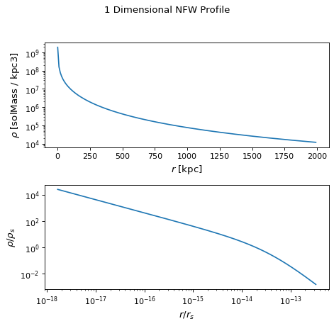
- Sample plots of an NFW profile with the following parameters are displayed below:
mass= \(2.0 x 10^{15} M_{sun}\)concentration= 8.5redshift= 0.63
The first plot is of the NFW profile density as a function of radius.
The second plot displays the profile density and radius normalized by the NFW scale
density and scale radius, respectively. The scale density and scale radius are available
as attributes rho_s and r_s, and the overdensity radius can be accessed via r_virial.
import numpy as np
import matplotlib.pyplot as plt
from astropy.modeling.models import NFW
import astropy.units as u
from astropy import cosmology

# NFW Parameters
mass = u.Quantity(2.0E15, u.M_sun)
concentration = 8.5
redshift = 0.63
cosmo = cosmology.Planck15
massfactor = ("critical", 200)

# Create NFW Object
n = NFW(mass=mass, concentration=concentration, redshift=redshift, cosmo=cosmo,
        massfactor=massfactor)

# Radial distribution for plotting
radii = range(1,2001,10) * u.kpc

# Radial NFW density distribution
n_result = n(radii)

# Plot creation
fig, axs = plt.subplots(nrows=2)
fig.suptitle('1 Dimensional NFW Profile')

# Density profile subplot
axs[0].plot(radii, n_result, '-')
axs[0].set(
    yscale='log',
    xlabel=fr"$r$ [{radii.unit}]",
    ylabel=fr"$\rho$ [{n_result.unit}]",
)

# Create scaled density / scaled radius subplot
# NFW Object
n = NFW(mass=mass, concentration=concentration, redshift=redshift, cosmo=cosmo,
        massfactor=massfactor)

# Radial distribution for plotting
radii = np.logspace(np.log10(1e-5), np.log10(2), num=1000) * u.Mpc
n_result = n(radii)

# Scaled density / scaled radius subplot
axs[1].plot(radii / n.radius_s, n_result / n.density_s, '-')
axs[1].set(
    xscale='log',
    yscale='log',
    xlabel=r"$r / r_s$",
    ylabel=r"$\rho / \rho_s$",
)

# Display plot
fig.tight_layout(rect=[0, 0.03, 1, 0.95])
plt.show()
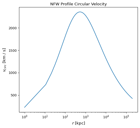
The circular_velocity() member provides the circular
velocity at each position r via the equation:
where x is the ratio r\(/r_{vir}\). Circular velocities are provided in km/s.
A sample plot of circular velocities of an NFW profile with the following parameters is displayed below:
mass= \(2.0 x 10^{15} M_{sun}\)
concentration= 8.5
redshift= 0.63
The maximum circular velocity and radius of maximum circular velocity are available as attributes
v_max and r_max.
import matplotlib.pyplot as plt
from astropy.modeling.models import NFW
import astropy.units as u
from astropy import cosmology

# NFW Parameters
mass = u.Quantity(2.0E15, u.M_sun)
concentration = 8.5
redshift = 0.63
cosmo = cosmology.Planck15
massfactor = ("critical", 200)

# Create NFW Object
n = NFW(mass=mass, concentration=concentration, redshift=redshift, cosmo=cosmo,
        massfactor=massfactor)

# Radial distribution for plotting
radii = range(1,200001,10) * u.kpc

# NFW circular velocity distribution
n_result = n.circular_velocity(radii)

# Plot creation
fig,ax = plt.subplots()
ax.set_title('NFW Profile Circular Velocity')
ax.plot(radii, n_result, '-')
ax.set_xscale('log')
ax.set_xlabel(fr"$r$ [{radii.unit}]")
ax.set_ylabel(r"$v_{circ}$" + f" [{n_result.unit}]")

# Display plot
plt.tight_layout(rect=[0, 0.03, 1, 0.95])
plt.show()
Cosmologies#
The instances of the Cosmology class (and subclasses) include
to_format(), a method to convert a Cosmology to another python
object. Specifically, any redshift method can be converted to a
FittableModel instance using the argument
format="astropy.model".
During the conversion, each Cosmology Parameter
is converted to a astropy.modeling.Model
Parameter, while the redshift-method becomes the
model’s __call__ / evaluate method.
This means cosmologies can now be fit with data!
>>> from astropy.cosmology import Planck18
>>> model = Planck18.to_format(format="astropy.model", method="lookback_time")
>>> model
<FlatLambdaCDMCosmologyLookbackTimeModel(H0=67.66 km / (Mpc s), Om0=0.30966,
    Tcmb0=2.7255 K, Neff=3.046, m_nu=[0.  , 0.  , 0.06] eV, Ob0=0.04897,
    name='Planck18')>
When finished, e.g. fitting, a model can be turned back into a Cosmology
using from_format().
>>> from astropy.cosmology import Cosmology
>>> cosmo = Cosmology.from_format(model, format="astropy.model")
>>> cosmo == Planck18
True