Lomb-Scargle Periodograms for Multiband Data

The Lomb-Scargle periodogram (after Lomb [1], and Scargle [2]) is a commonly used statistical tool designed to detect periodic signals in unevenly spaced observations. The base LombScargle provides an interface for several implementations of the Lomb-Scargle periodogram. However, LombScargle only handles a single band of data. The LombScargleMultiband class adapts this interface to handle multiband data (where multiple bands/filters are present).

The code here is adapted from the astroml package ([3], [4]) and the gatspy package ([5], [6]), but conforms closely to the design paradigms established in LombScargle. For a detailed practical discussion of the Multiband Lomb-Scargle periodogram, which guided the development of this class, see Periodograms for Multiband Astronomical Time Series [6].

Basic Usage

Note

As in LombScargle, frequencies in LombScargleMultiband are not angular frequencies, but rather frequencies of oscillation (i.e., number of cycles per unit time).

The Lomb-Scargle Multiband periodogram is designed to detect periodic signals in unevenly spaced observations with multiple bands of data present.

Example

To detect periodic signals in unevenly spaced observations, consider the following multiband data, where 5 bands (u, g, r, i, and z) have 60 datapoints each.

>>> import numpy as np
>>> t = []
>>> y = []
>>> bands = []
>>> dy = []
>>> N=60
>>> for i, band in enumerate(['u','g','r','i','z']):
...     rng = np.random.default_rng(i)
...     t_band = 300 * rng.random(N)
...     y_band = 3 + 2 * np.sin(2 * np.pi * t_band)
...     dy_band = 0.01 * (0.5 + rng.random(N)) # uncertainties
...     y_band += dy_band * rng.standard_normal(N)
...     t += list(t_band)
...     y += list(y_band)
...     dy += list(dy_band)
...     bands += [band] * N

The Lomb-Scargle periodogram, evaluated at frequencies chosen automatically based on the input data, can be computed as follows using the LombScargleMultiband class, with the bands argument being the sole difference in comparison to the LombScargle interface:

>>> from astropy.timeseries import LombScargleMultiband
>>> frequency,power = LombScargleMultiband(t, y, bands, dy).autopower()

Plotting the result with Matplotlib gives:

(png, svg, pdf)

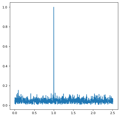
The periodogram shows a clear spike at a frequency of 1 cycle per unit time, as we would expect from the data we constructed. The resulting power is a single array, with combined input from each of the bands dependent upon the implementation chosen in the method keyword.

Periodograms from TimeSeries objects

LombScargleMultiband is able to operate on TimeSeries objects, provided the TimeSeries object meets a formatting requirement. The requirement is that the flux (or magnitudes) and errors for each band are provided in separate columns. If instead, your TimeSeries object has a singular flux column with an associated band label column, these columns may be passed directly to LombScargleMultiband as 1-d arrays.

Example

Consider the following generator code for a TimeSeries object where timeseries data is populated for three photometric bands (g,r,i).

>>> from astropy.timeseries import LombScargleMultiband, TimeSeries
>>> from astropy.table import MaskedColumn
>>> import numpy as np
>>> import astropy.units as u

>>> rng = np.random.default_rng(1)
>>> deltas = 240 * rng.random(180)
>>> ts1 = TimeSeries(time_start="2011-01-01T00:00:00",
...                  time_delta=deltas*u.minute)

>>> # g band fluxes
>>> g_flux = [0] * 180 * u.mJy
>>> g_err = [0] * 180 * u.mJy
>>> y_g = np.round(3 + 2 * np.sin(10 * np.pi * ts1['time'].mjd[0:60]),3)
>>> dy_g = np.round(0.01 * (0.5 + rng.random(60)), 3) # uncertainties
>>> g_flux.value[0:60] = y_g
>>> g_err.value[0:60] = dy_g
>>> ts1["g_flux"]  = MaskedColumn(g_flux, mask=[False]*60+[True]*120)
>>> ts1["g_err"]  = MaskedColumn(g_err, mask=[False]*60+[True]*120)
>>> # r band fluxes
>>> r_flux = [0] * 180 * u.mJy
>>> r_err = [0] * 180 * u.mJy
>>> y_r = np.round(3 + 2 * np.sin(10 * np.pi * ts1['time'].mjd[60:120]),3)
>>> dy_r = np.round(0.01 * (0.5 + rng.random(60)), 3) # uncertainties
>>> r_flux.value[60:120] = y_r
>>> r_err.value[60:120] = dy_r
>>> ts1['r_flux'] = MaskedColumn(r_flux, mask=[True]*60+[False]*60+[True]*60)
>>> ts1['r_err'] = MaskedColumn(r_err, mask=[True]*60+[False]*60+[True]*60)
>>> # i band fluxes
>>> i_flux = [0] * 180 * u.mJy
>>> i_err = [0] * 180 * u.mJy
>>> y_i = np.round(3 + 2 * np.sin(10 * np.pi * ts1['time'].mjd[120:]),3)
>>> dy_i = np.round(0.01 * (0.5 + rng.random(60)), 3) # uncertainties
>>> i_flux.value[120:] = y_i
>>> i_err.value[120:] = dy_i
>>> ts1["i_flux"]  = MaskedColumn(i_flux, mask=[True]*120+[False]*60)
>>> ts1["i_err"]  = MaskedColumn(i_err, mask=[True]*120+[False]*60)
>>> ts1
<TimeSeries length=180>
          time           g_flux  g_err   r_flux  r_err   i_flux  i_err
                          mJy     mJy     mJy     mJy     mJy     mJy
          Time          float64 float64 float64 float64 float64 float64
----------------------- ------- ------- ------- ------- ------- -------
2011-01-01T00:00:00.000     3.0   0.012     ———     ———     ———     ———
2011-01-01T02:02:50.231   3.891   0.009     ———     ———     ———     ———
2011-01-01T05:50:56.909   4.961   0.007     ———     ———     ———     ———
2011-01-01T06:25:32.807   4.697   0.014     ———     ———     ———     ———
2011-01-01T10:13:13.359   4.451   0.005     ———     ———     ———     ———
2011-01-01T11:28:03.732   4.283   0.008     ———     ———     ———     ———
2011-01-01T13:09:39.633   1.003   0.015     ———     ———     ———     ———
2011-01-01T16:28:18.550   3.833   0.008     ———     ———     ———     ———
2011-01-01T18:06:31.018    1.02   0.013     ———     ———     ———     ———
                    ...     ...     ...     ...     ...     ...     ...
2011-01-15T16:03:17.207     ———     ———     ———     ———   4.656   0.014
2011-01-15T17:29:38.139     ———     ———     ———     ———   1.423    0.01
2011-01-15T20:03:35.935     ———     ———     ———     ———   4.805   0.008
2011-01-15T21:35:02.069     ———     ———     ———     ———   3.042   0.007
2011-01-15T23:06:35.567     ———     ———     ———     ———   1.162    0.01
2011-01-16T01:07:30.330     ———     ———     ———     ———    4.99   0.009
2011-01-16T01:11:31.138     ———     ———     ———     ———     5.0   0.011
2011-01-16T03:09:58.569     ———     ———     ———     ———   1.314    0.01
2011-01-16T07:03:09.586     ———     ———     ———     ———   3.383   0.005

Our timeseries data is set up to be asynchronous, where a given timestamp corresponds to a measurement in a single band. However, if your data instead has one timestamp per multiple band measurements, or a mixture, LombScargleMultiband will still be able to operate on it.

To operate on the example TimeSeries, LombScargleMultiband has a loader function, as follows:

>>> ls = LombScargleMultiband.from_timeseries(ts1, signal_column=['g_flux', 'r_flux', 'i_flux'],
...                                           uncertainty_column=['g_err', 'r_err', 'i_err'],
...                                           band_labels=['g', 'r', 'i'])

signal_column requires a list of columns that correspond to the flux or magnitude measurements in each band. uncertainty_column and band_labels are optional, but if specified must be lists of equal size to signal_column. uncertainty_column specifies the columns containing the associated errors per band, while band_labels provides the labels to use for each photometric band. From here, LombScargleMultiband can be worked with as normal. For example:

>>> frequency,power = ls.autopower()

Consistencies with LombScargle

LombScargleMultiband is an inherited class of LombScargle, and was developed to provide as similar of an interface to LombScargle as possible. From this, there are several core aspects of LombScargle that remain true for LombScargleMultiband.

Measurement Uncertainties

The LombScargleMultiband interface can also handle data with measurement uncertainties. As shown in the example above.

Periodograms and Units

The LombScargleMultiband interface properly handles Quantity objects with units attached, and will validate the inputs to make sure units are appropriate.

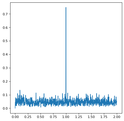
Specifying the Frequency Grid

As shown above, the autopower() method automatically determines a frequency grid, using autofrequency(). The tunable parameters are identical to those shown for LombScargle. And likewise, a custom frequency grid may be supplied directly to the power() function.

Example

>>> frequency = np.linspace(0, 2, 1000)
>>> power = LombScargleMultiband(t, y, bands, dy).power(frequency)

(png, svg, pdf)

Periodogram Implementations

Two implementations of the Multiband Lomb-Scargle Periodogram are available within LombScargleMultiband, flexible and fast, which are selectable via the power() method’s method parameter. flexible is a direct port of the LombScargleMultiband algorithm used in the gatspy gatspy package. It constructs a common model, and an offset model per individual band. It then applies regularization to the resulting model to constrain complexity, resulting in a flexible model for any given multiband timeseries dataset. As it’s name implies, fast is potentially quicker alternative that fits each band independently and combines them by weight. The independent band-by-band fits leverage LombScargle. As a result the sb_method parameter is available in power() to choose the single-band method used in power() for each band. Keep in mind that the speed of fast is dependent on the underlying speed of the choice of sb_method.

Example

flexible:

>>> frequency, power = LombScargleMultiband(t,y,bands,dy).autopower(method='flexible')

fast, with fast also chosen as the power() method:

>>> frequency, power = LombScargleMultiband(t,y,bands,dy).autopower(method='fast', sb_method='fast')

The Multiband Lomb-Scargle Model

The model() method fits a sinusoidal model to the data at a chosen frequency. The sinusoidal model complexity is tunable via the nterms_base and nterms_band parameters. These control the number of sinusoidal terms available to the base model (common to all bands) and the number of sinusoidal terms available to each bands offset model.

Note

Either of nterms_base and nterms_band may be set to 0, though not both. The case when nterms_base =0 and nterms_band =1 is a special case referred to as the multi-phase model, where the base model is reduced to a simple offset, and therefore the bands are solved independently (a single-band fit). Further discussed in Periodograms for Multiband Astronomical Time Series [6]

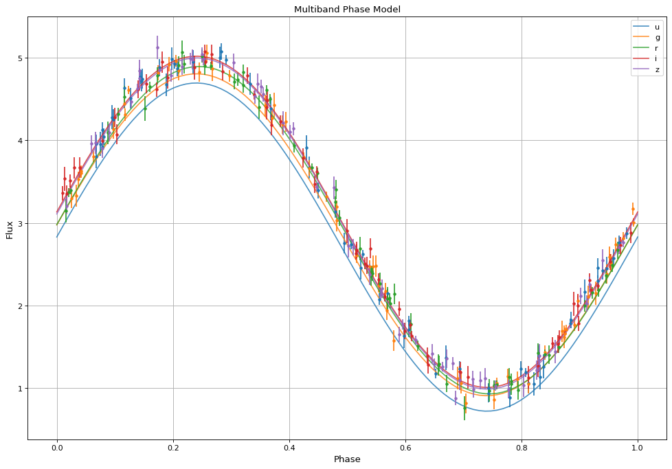
Example

The following example uses the same data as above. autopower() is used to return the periodogram, and we can select the frequency at which the power is maximum for our model:

>>> model = LombScargleMultiband(t, y, bands, dy, nterms_base=1, nterms_band=1)
>>> frequency, power = model.autopower(method='flexible')
>>> freq_maxpower = frequency[np.argmax(power)]

We can then model based on the found frequency, and time (phased by the frequency):

>>> t_phase = np.linspace(0, 1/freq_maxpower, 100)
>>> y_fit = model.model(t_phase, freq_maxpower)

The resulting fit is then of shape (number of bands, number of timesteps), or (5,100) in this particular case. By plotting the result, we see the model has recovered the expected sinusoid recovered at the correct frequency:

(png, svg, pdf)

False Alarm Probabilities

Unlike LombScargle, LombScargleMultiband does not have False Alarm Probabilities implemented. The algorithms available for LombScargle are valid only for single term periodograms, which is rarely valid for models in the Multiband case.

Literature References

[1]

Lomb, N.R. Least-squares frequency analysis of unequally spaced data. Ap&SS 39 pp. 447-462 (1976)

[2]

Scargle, J. D. Studies in astronomical time series analysis. II - Statistical aspects of spectral analysis of unevenly spaced data. ApJ 1:263 pp. 835-853 (1982)

[3]

Vanderplas, J., Connolly, A. Ivezic, Z. & Gray, A. Introduction to astroML: Machine learning for astrophysics. Proceedings of the Conference on Intelligent Data Understanding (2012)

[4]

Vanderplas, J., Connolly, A. Ivezic, Z. & Gray, A. Statistics, Data Mining and Machine Learning in Astronomy. Princeton Press (2014)}

[5]

VanderPlas, J. Gatspy: General Tools for Astronomical Time Series in Python (2015) https://zenodo.org/record/14833

[6] (1,2,3)

VanderPlas, J. & Ivezic, Z. Periodograms for Multiband Astronomical Time Series. ApJ 812.1:18 (2015)