Uncertainties and Distributions (astropy.uncertainty)#
Introduction#
Note
This subpackage is still in development.
astropy provides a Distribution object to represent statistical
distributions in a form that acts as a drop-in replacement for a Quantity
object or a regular numpy.ndarray. Used in this manner, Distribution provides
uncertainty propagation at the cost of additional computation. It can also more
generally represent sampled distributions for Monte Carlo calculation
techniques, for instance.
The core object for this feature is the Distribution. Currently, all
such distributions are Monte Carlo sampled. While this means each distribution
may take more memory, it allows arbitrarily complex operations to be performed
on distributions while maintaining their correlation structure. Some specific
well-behaved distributions (e.g., the normal distribution) have
analytic forms which may eventually enable a more compact and efficient
representation. In the future, these may provide a coherent uncertainty
propagation mechanism to work with NDData. However, this is
not currently implemented. Hence, details of storing uncertainties for
NDData objects can be found in the N-Dimensional Datasets (astropy.nddata)
section.
Getting Started#
To demonstrate a basic use case for distributions, consider the problem of uncertainty propagation of normal distributions. Assume there are two measurements you wish to add, each with normal uncertainties. We start with some initial imports and setup:
>>> import numpy as np
>>> from astropy import units as u
>>> from astropy import uncertainty as unc
>>> rng = np.random.default_rng(12345)  # ensures reproducible example numbers
Now we create two Distribution objects to represent our distributions:
>>> a = unc.normal(1*u.kpc, std=30*u.pc, n_samples=10000)
>>> b = unc.normal(2*u.kpc, std=40*u.pc, n_samples=10000)
For normal distributions, the centers should add as expected, and the standard
deviations add in quadrature. We can check these results (to the limits of our
Monte Carlo sampling) trivially with Distribution arithmetic and attributes:
>>> c = a + b
>>> c
<QuantityDistribution [...] kpc with n_samples=10000>
>>> c.pdf_mean()
<Quantity 2.99970555 kpc>
>>> c.pdf_std().to(u.pc)
<Quantity 50.07120457 pc>
Indeed these are close to the expectations. While this may seem unnecessary for
the basic Gaussian case, for more complex distributions or arithmetic
operations where error analysis becomes untenable, Distribution still powers
through:
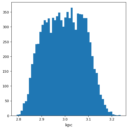
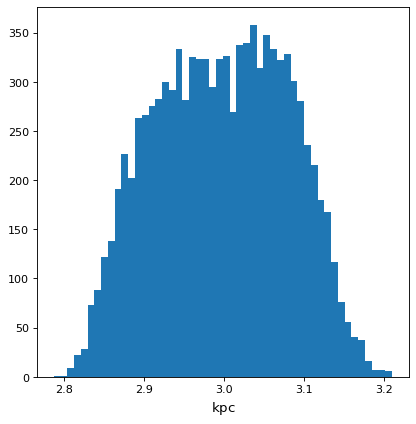
>>> d = unc.uniform(center=3*u.kpc, width=800*u.pc, n_samples=10000)
>>> e = unc.Distribution(((rng.beta(2,5, 10000)-(2/7))/2 + 3)*u.kpc)
>>> f = (c * d * e) ** (1/3)
>>> f.pdf_mean()
<Quantity 2.99760998 kpc>
>>> f.pdf_std()
<Quantity 0.08308941 kpc>
>>> from matplotlib import pyplot as plt
>>> from astropy.visualization import quantity_support
>>> with quantity_support():
...     fig, ax = plt.subplots()
...     ax.hist(f.distribution, bins=50)
Using astropy.uncertainty#
Creating Distributions#
The most direct way to create a distribution is to use an array or Quantity
that carries the samples in the last dimension:
>>> import numpy as np
>>> from astropy import units as u
>>> from astropy import uncertainty as unc
>>> rng = np.random.default_rng(123456)  # ensures "random" numbers match examples below
>>> unc.Distribution(rng.poisson(12, (1000)))
NdarrayDistribution([..., 12,...]) with n_samples=1000
>>> pq = rng.poisson([1, 5, 30, 400], (1000, 4)).T * u.ct # note the transpose, required to get the sampling on the *last* axis
>>> distr = unc.Distribution(pq)
>>> distr
<QuantityDistribution [[...],
           [...],
           [...],
           [...]] ct with n_samples=1000>
Note the distinction for these two distributions: the first is built from an
array and therefore does not have Quantity attributes like unit, while the
latter does have these attributes. This is reflected in how they interact with
other objects, for example, the NdarrayDistribution will not combine with
Quantity objects containing units.
For commonly used distributions, helper functions exist to make creating them more convenient. The examples below demonstrate several equivalent ways to create a normal/Gaussian distribution:
>>> center = [1, 5, 30, 400]
>>> n_distr = unc.normal(center*u.kpc, std=[0.2, 1.5, 4, 1]*u.kpc, n_samples=1000)
>>> n_distr = unc.normal(center*u.kpc, var=[0.04, 2.25, 16, 1]*u.kpc**2, n_samples=1000)
>>> n_distr = unc.normal(center*u.kpc, ivar=[25, 0.44444444, 0.625, 1]*u.kpc**-2, n_samples=1000)
>>> n_distr.distribution.shape
(4, 1000)
>>> unc.normal(center*u.kpc, std=[0.2, 1.5, 4, 1]*u.kpc, n_samples=100).distribution.shape
(4, 100)
>>> unc.normal(center*u.kpc, std=[0.2, 1.5, 4, 1]*u.kpc, n_samples=20000).distribution.shape
(4, 20000)
Additionally, Poisson and uniform Distribution creation functions exist:
>>> unc.poisson(center*u.count, n_samples=1000)
<QuantityDistribution [[...],
             [...],
             [...],
             [...]] ct with n_samples=1000>
>>> uwidth = [10, 20, 10, 55]*u.pc
>>> unc.uniform(center=center*u.kpc, width=uwidth, n_samples=1000)
<QuantityDistribution [[...],
             [...],
             [...],
             [...]] kpc with n_samples=1000>
>>> unc.uniform(lower=center*u.kpc - uwidth/2,  upper=center*u.kpc + uwidth/2, n_samples=1000)
<QuantityDistribution [[...],
             [...],
             [...],
             [...]] kpc with n_samples=1000>
Users are free to create their own distribution classes following similar patterns.
Using Distributions#
This object now acts much like a Quantity or numpy.ndarray for all but the
non-sampled dimension, but with additional statistical operations that work on
the sampled distributions:
>>> distr.shape
(4,)
>>> distr.size
4
>>> distr.unit
Unit("ct")
>>> distr.n_samples
1000
>>> distr.pdf_mean()
<Quantity [  1.034,   5.026,  29.994, 400.365] ct>
>>> distr.pdf_std()
<Quantity [ 1.04539179,  2.19484031,  5.47776998, 19.87022333] ct>
>>> distr.pdf_var()
<Quantity [  1.092844,   4.817324,  30.005964, 394.825775] ct2>
>>> distr.pdf_median()
<Quantity [   1.,   5.,  30., 400.] ct>
>>> distr.pdf_mad()  # Median absolute deviation
<Quantity [ 1.,  1.,  4., 13.] ct>
>>> distr.pdf_smad()  # Median absolute deviation, rescaled to match std for normal
<Quantity [ 1.48260222,  1.48260222,  5.93040887, 19.27382884] ct>
>>> distr.pdf_percentiles([10, 50, 90])
<Quantity [[  0. ,   2. ,  23. , 375. ],
           [  1. ,   5. ,  30. , 400. ],
           [  2. ,   8. ,  37. , 426.1]] ct>
>>> distr.pdf_percentiles([.1, .5, .9]*u.dimensionless_unscaled)
<Quantity [[  0. ,   2. ,  23. , 375. ],
          [  1. ,   5. ,  30. , 400. ],
          [  2. ,   8. ,  37. , 426.1]] ct>
If need be, the underlying array can then be accessed from the distribution
attribute:
>>> distr.distribution
<Quantity [[  2.,   2.,   0., ...,   1.,   0.,   1.],
           [  3.,   2.,   8., ...,   8.,   3.,   3.],
           [ 31.,  30.,  32., ...,  20.,  34.,  31.],
           [354., 373., 384., ..., 410., 404., 395.]] ct>
>>> distr.distribution.shape
(4, 1000)
A Quantity distribution interacts naturally with non-Distribution
Quantity objects, assuming the Quantity is a Dirac delta distribution:
>>> distr_in_kpc = distr * u.kpc/u.count  # for the sake of round numbers in examples
>>> distrplus = distr_in_kpc + [2000,0,0,500]*u.pc
>>> distrplus.pdf_median()
<Quantity [   3. ,   5. ,  30. , 400.5] kpc>
>>> distrplus.pdf_var()
<Quantity [  1.092844,   4.817324,  30.005964, 394.825775] kpc2>
It also operates as expected with other distributions (but see below for a discussion of covariances):
>>> means = [2000, 0, 0, 500]
>>> sigmas = [1000, .01, 3000, 10]
>>> another_distr = unc.Distribution((rng.normal(means, sigmas, (1000,4))).T * u.pc)
>>> combined_distr = distr_in_kpc + another_distr
>>> combined_distr.pdf_median()
<Quantity [  2.81374275,   4.99999631,  29.7150889 , 400.49576691] kpc>
>>> combined_distr.pdf_var()
<Quantity [  2.15512118,   4.817324  ,  39.0614616 , 394.82969655] kpc2>
Covariance in Distributions and Discrete Sampling Effects#
One of the main applications for distributions is uncertainty propagation, which
critically requires proper treatment of covariance. This comes naturally in the
Monte Carlo sampling approach used by the Distribution class, as long as
proper care is taken with sampling error.
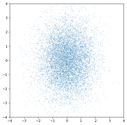
To start with a basic example, two un-correlated distributions should produce an un-correlated joint distribution plot:
>>> import numpy as np
>>> from astropy import units as u
>>> from astropy import uncertainty as unc
>>> from matplotlib import pyplot as plt
>>> n1 = unc.normal(center=0., std=1, n_samples=10000)
>>> n2 = unc.normal(center=0., std=2, n_samples=10000)
>>> fig, ax = plt.subplots()
>>> ax.scatter(n1.distribution, n2.distribution, s=2, lw=0, alpha=.5)
>>> ax.set(xlim=(-4, 4), ylim=(-4, 4))
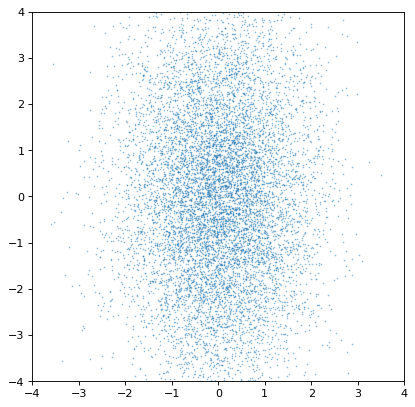
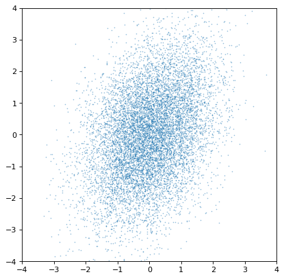
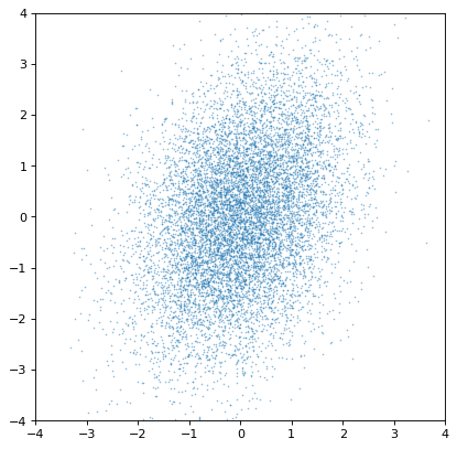
Indeed, the distributions are independent. If we instead construct a covariant pair of Gaussians, it is immediately apparent:
>>> rng = np.random.default_rng(357)
>>> ncov = rng.multivariate_normal([0, 0], [[1, .5], [.5, 2]], size=10000)
>>> n1 = unc.Distribution(ncov[:, 0])
>>> n2 = unc.Distribution(ncov[:, 1])
>>> plt.scatter(n1.distribution, n2.distribution, s=2, lw=0, alpha=.5)
>>> plt.xlim(-4, 4)
>>> plt.ylim(-4, 4)
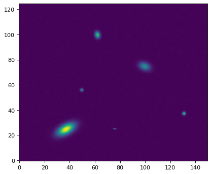
Most importantly, the proper correlated structure is preserved or generated as expected by appropriate arithmetic operations. For example, ratios of uncorrelated normal distribution gain covariances if the axes are not independent, as in this simulation of iron, hydrogen, and oxygen abundances in a hypothetical collection of stars:
>>> fe_abund = unc.normal(center=-2, std=.25, n_samples=10000)
>>> o_abund = unc.normal(center=-6., std=.5, n_samples=10000)
>>> h_abund = unc.normal(center=-0.7, std=.1, n_samples=10000)
>>> feh = fe_abund - h_abund
>>> ofe = o_abund - fe_abund
>>> plt.scatter(ofe.distribution, feh.distribution, s=2, lw=0, alpha=.5)
>>> plt.xlabel('[Fe/H]')
>>> plt.ylabel('[O/Fe]')
This demonstrates that the correlations naturally arise from the variables, but there is no need to explicitly account for it: the sampling process naturally recovers correlations that are present.
An important note of warning, however, is that the covariance is only preserved if the sampling axes are exactly matched sample by sample. If they are not, all covariance information is (silently) lost:
>>> n2_wrong = unc.Distribution(ncov[::-1, 1])  #reverse the sampling axis order
>>> plt.scatter(n1.distribution, n2_wrong.distribution, s=2, lw=0, alpha=.5)
>>> plt.xlim(-4, 4)
>>> plt.ylim(-4, 4)
Moreover, an insufficiently sampled distribution may give poor estimates or hide correlations. The example below is the same as the covariant Gaussian example above, but with 200x fewer samples:
>>> ncov = rng.multivariate_normal([0, 0], [[1, .5], [.5, 2]], size=50)
>>> n1 = unc.Distribution(ncov[:, 0])
>>> n2 = unc.Distribution(ncov[:, 1])
>>> plt.scatter(n1.distribution, n2.distribution, s=5, lw=0)
>>> plt.xlim(-4, 4)
>>> plt.ylim(-4, 4)
>>> np.cov(n1.distribution, n2.distribution)
array([[0.95534365, 0.35220031],
       [0.35220031, 1.99511743]])
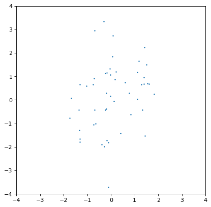
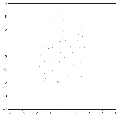
The covariance structure is much less apparent by eye, and this is reflected in significant discrepancies between the input and output covariance matrix. In general this is an intrinsic trade-off using sampled distributions: a smaller number of samples is computationally more efficient, but leads to larger uncertainties in any of the relevant quantities. These tend to be of order \(\sqrt{n_{\rm samples}}\) in any derived quantity, but that depends on the complexity of the distribution in question.
Reference/API#
astropy.uncertainty Package#
This sub-package contains classes and functions for creating distributions that
work similar to Quantity or array objects, but can propagate
uncertainties.
Functions#
Classes#
|
A scalar value or array values with associated uncertainty distribution. |