Robust Statistical Estimators#
Robust statistics provides reliable estimates of basic statistics for complex distributions. The statistics package includes several robust statistical functions that are commonly used in astronomy. This includes methods for rejecting outliers as well as statistical description of the underlying distributions.
In addition to the functions mentioned here, models can be fit with outlier
rejection using FittingWithOutlierRemoval().
Sigma Clipping#
Sigma clipping provides a fast method for identifying outliers in a distribution. For a distribution of points, a center and a standard deviation are calculated. Values which are less or more than a specified number of standard deviations from a center value are rejected. The process can be iterated to further reject outliers.
The astropy.stats package provides both a functional and
object-oriented interface for sigma clipping. The function is called
sigma_clip() and the class is called
SigmaClip. By default, they both return a
masked array where the rejected points are masked.
Examples#
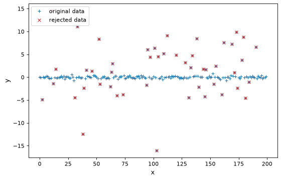
We can start by generating some data that has a mean of 0 and standard deviation of 0.2, but with outliers:
>>> import numpy as np
>>> import scipy.stats as stats
>>> rng = np.random.default_rng(0)
>>> x = np.arange(200)
>>> y = np.zeros(200)
>>> c = stats.bernoulli.rvs(0.35, size=x.shape)
>>> y += (rng.normal(0., 0.2, x.shape) +
...       c * rng.normal(3.0, 5.0, x.shape))
Now we can use sigma_clip() to perform sigma
clipping on the data:
>>> from astropy.stats import sigma_clip
>>> filtered_data = sigma_clip(y, sigma=3, maxiters=10)
The output masked array then can be used to calculate statistics on the data, fit models to the data, or otherwise explore the data.
To perform the same sigma clipping with the
SigmaClip class:
>>> from astropy.stats import SigmaClip
>>> sigclip = SigmaClip(sigma=3, maxiters=10)
>>> print(sigclip)
<SigmaClip>
   sigma: 3
   sigma_lower: None
   sigma_upper: None
   maxiters: 10
   cenfunc: <function median at 0x108dbde18>
   stdfunc: <function std at 0x103ab52f0>
>>> filtered_data = sigclip(y)
Note that once the sigclip instance is defined above, it can be
applied to other data using the same already defined sigma-clipping
parameters.
For basic statistics, sigma_clipped_stats() is a
convenience function to calculate the sigma-clipped mean, median, and
standard deviation of an array. As can be seen, rejecting the
outliers returns accurate values for the underlying distribution.
To use sigma_clipped_stats() for sigma-clipped statistics
calculation:
>>> from astropy.stats import sigma_clipped_stats
>>> y.mean(), np.median(y), y.std()
(np.float64(0.7068938765410144), np.float64(0.013567387681385379), np.float64(3.599605215851649))
>>> sigma_clipped_stats(y, sigma=3, maxiters=10)
(np.float64(-0.0228473012826993), np.float64(-0.02356858871405204), np.float64(0.2079616996908159))
SigmaClippedStats is a
convenience class that extends the functionality of
sigma_clipped_stats():
>>> from astropy.stats import SigmaClippedStats
>>> stats = SigmaClippedStats(y, sigma=3, maxiters=10)
>>> stats.mean(), stats.median(), stats.std()
(np.float64(-0.0228473012826993), np.float64(-0.02356858871405204), np.float64(0.2079616996908159))
>>> stats.mode(), stats.var(), stats.mad_std()
(np.float64(-0.025011163576757534), np.float64(0.043248068538293126), np.float64(0.21277510956855722))
>>> stats.biweight_location(), stats.biweight_scale()
(np.float64(-0.0183718864859565), np.float64(0.21730062377965248))
sigma_clip() and
SigmaClip can be combined with other robust
statistics to provide improved outlier rejection as well.
import numpy as np
import scipy.stats as stats
from matplotlib import pyplot as plt
from astropy.stats import sigma_clip, mad_std

# Generate fake data that has a mean of 0 and standard deviation of 0.2 with outliers
rng = np.random.default_rng(0)
x = np.arange(200)
y = np.zeros(200)
c = stats.bernoulli.rvs(0.35, size=x.shape)
y += (rng.normal(0., 0.2, x.shape) +
      c * rng.normal(3.0, 5.0, x.shape))

filtered_data = sigma_clip(y, sigma=3, maxiters=1, stdfunc=mad_std)

# plot the original and rejected data
fig, ax = plt.subplots(figsize=(8, 5))
ax.plot(x, y, '+', color='#1f77b4', label="original data")
ax.plot(x[filtered_data.mask], y[filtered_data.mask], 'x',
         color='#d62728', label="rejected data")
ax.set(xlabel='x', ylabel='y')
ax.legend(loc=2, numpoints=1)
astropy.stats.sigma_clipping Module#
Functions#
|
Perform sigma-clipping on the provided data. |
|
Calculate sigma-clipped statistics on the provided data. |
Classes#
|
Class to perform sigma clipping. |
|
Class to calculate sigma-clipped statistics on the provided data. |
Class Inheritance Diagram#
Median Absolute Deviation#
The median absolute deviation (MAD) is a measure of the spread of a
distribution and is defined as median(abs(a - median(a))). The
MAD can be calculated using median_absolute_deviation. For a
normal distribution, the MAD is related to the standard deviation by a factor
of 1.4826, and a convenience function, mad_std, is
available to apply the conversion.
Note
A function can be supplied to the
median_absolute_deviation to specify the median
function to be used in the calculation. Depending on the version
of NumPy and whether the array is masked or contains irregular
values, significant performance increases can be had by
preselecting the median function. If the median function is not
specified, median_absolute_deviation will attempt
to select the most relevant function according to the input data.
Biweight Estimators#
A set of functions are included in the astropy.stats package that use the
biweight formalism. These functions have long been used in astronomy,
particularly to calculate the velocity dispersion of galaxy clusters [1]. The
following set of tasks are available for biweight measurements:
astropy.stats.biweight Module#
This module contains functions for computing robust statistics using Tukey’s biweight function.
Functions#
|
Compute the biweight location. |
|
Compute the biweight midcorrelation between two variables. |
|
Compute the biweight midcovariance between pairs of multiple variables. |
|
Compute the biweight midvariance. |
|
Compute the biweight scale. |