Overplotting markers and artists#
The class WCSAxes provides two handy methods:
plot_coord(),
scatter_coord()
Used to plots and scatter respectively SkyCoord or BaseCoordinateFrame coordinates on the axes. The transform keyword argument will be created based on the coordinate, specifying it here will throw a TypeError.
For the example in the following page we start from the example introduced in Initializing axes with world coordinates.
Pixel coordinates#
Apart from the handling of the ticks, tick labels, and grid lines, the
WCSAxes class behaves like a normal Matplotlib
Axes instance, and methods such as
imshow(),
contour(),
plot(),
scatter(), and so on will work and plot the
data in pixel coordinates by default.
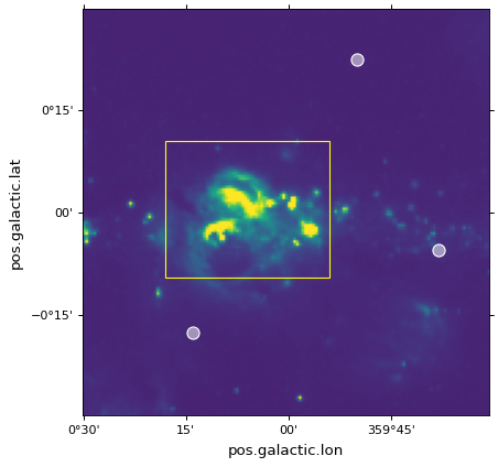
In the following example, the scatter markers and the rectangle will be plotted in pixel coordinates:
# The following line makes it so that the zoom level no longer changes,
# otherwise Matplotlib has a tendency to zoom out when adding overlays.
ax.set_autoscale_on(False)

# Add a rectangle with bottom left corner at pixel position (30, 50) with a
# width and height of 60 and 50 pixels respectively.
from matplotlib.patches import Rectangle
r = Rectangle((30., 50.), 60., 50., edgecolor='yellow', facecolor='none')
ax.add_patch(r)

# Add three markers at (40, 30), (100, 130), and (130, 60). The facecolor is
# a transparent white (0.5 is the alpha value).
ax.scatter([40, 100, 130], [30, 130, 60], s=100, edgecolor='white', facecolor=(1, 1, 1, 0.5))
World coordinates#
All such Matplotlib commands allow a transform= argument to be passed,
which will transform the input from world to pixel coordinates before it is
passed to Matplotlib and plotted. For instance:
ax.scatter(..., transform=...)
will take the values passed to scatter() and will
transform them using the transformation passed to transform=, in order to
end up with the final pixel coordinates.
The WCSAxes class includes a get_transform()
method that can be used to get the appropriate transformation object to convert
from various world coordinate systems to the final display coordinate system
required by Matplotlib. The get_transform() method can
take a number of different inputs, which are described in this and subsequent
sections. The two simplest inputs to this method are 'world' and
'pixel'.
For example, if your WCS defines an image where the coordinate system consists of an angle in degrees and a wavelength in nanometers, you can do:
ax.scatter([34], [3.2], transform=ax.get_transform('world'))
to plot a marker at (34deg, 3.2nm).
Using ax.get_transform('pixel') is equivalent to not using any
transformation at all (and things then behave as described in the Pixel
coordinates section).
Celestial coordinates#
For the special case where the WCS represents celestial coordinates, a number
of other inputs can be passed to get_transform(). These
are:
'fk4': B1950 FK4 equatorial coordinates'fk5': J2000 FK5 equatorial coordinates'icrs': ICRS equatorial coordinates'galactic': Galactic coordinates
In addition, any valid astropy.coordinates coordinate frame can be passed.
For example, you can add markers with positions defined in the FK5 system using:
ax.scatter(266.78238, -28.769255, transform=ax.get_transform('fk5'), s=300,
           edgecolor='white', facecolor='none')
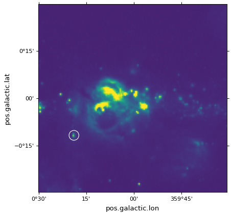
In the case of scatter() and plot(), the positions of the center of the markers is transformed, but the markers themselves are drawn in the frame of reference of the image, which means that they will not look distorted.
Patches/shapes/lines#
Transformations can also be passed to Astropy or Matplotlib patches. For example, we can
use the get_transform() method above to plot a quadrangle
in FK5 equatorial coordinates:
from astropy import units as u
from astropy.visualization.wcsaxes import Quadrangle

r = Quadrangle((266.0, -28.9)*u.deg, 0.3*u.deg, 0.15*u.deg,
               edgecolor='green', facecolor='none',
               transform=ax.get_transform('fk5'))
ax.add_patch(r)
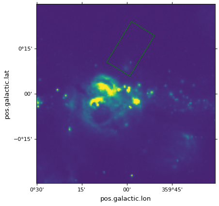
In this case, the quadrangle will be plotted at FK5 J2000 coordinates (266deg, -28.9deg).
See the Quadrangles section for more information on Quadrangle.
However, it is very important to note that while the height will indeed be 0.15 degrees, the width will not strictly represent 0.3 degrees on the sky, but an interval of 0.3 degrees in longitude (which, depending on the latitude, will represent a different angle on the sky).
In other words, if the width and height are set to the same value, the resulting polygon will not be a square.
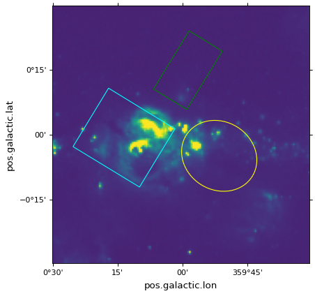
The same applies to the Circle patch, which will not actually produce a circle:
from matplotlib.patches import Circle

r = Quadrangle((266.4, -28.9)*u.deg, 0.3*u.deg, 0.3*u.deg,
               edgecolor='cyan', facecolor='none',
               transform=ax.get_transform('fk5'))
ax.add_patch(r)

c = Circle((266.4, -29.1), 0.15, edgecolor='yellow', facecolor='none',
           transform=ax.get_transform('fk5'))
ax.add_patch(c)
Important
If what you are interested is simply plotting circles around
sources to highlight them, then we recommend using
scatter(), since for the circular
marker (the default), the circles will be guaranteed to be
circles in the plot, and only the position of the center is
transformed.
To plot ‘true’ spherical circles, see the Spherical patches section.
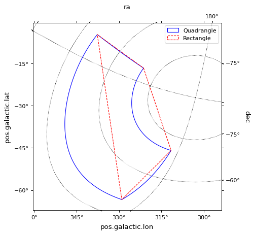
Quadrangles#
Quadrangle is the recommended patch for plotting a quadrangle, as opposed to Matplotlib’s Rectangle.
The edges of a quadrangle lie on two lines of constant longitude and two lines of constant latitude (or the equivalent component names in the coordinate frame of interest, such as right ascension and declination).
The edges of Quadrangle will render as curved lines if appropriate for the WCS transformation.
In contrast, Rectangle will always have straight edges.
Here’s a comparison of the two types of patches for plotting a quadrangle in ICRS coordinates on Galactic axes:
from matplotlib.patches import Rectangle

# Set the Galactic axes such that the plot includes the ICRS south pole
fig, ax = plt.subplots(subplot_kw=dict(projection=wcs))
ax.set_xlim(0, 10000)
ax.set_ylim(-10000, 0)

# Overlay the ICRS coordinate grid
overlay = ax.get_coords_overlay('icrs')
overlay.grid(color='black', ls='dotted')

# Add a quadrangle patch (100 degrees by 20 degrees)
q = Quadrangle((255, -70)*u.deg, 100*u.deg, 20*u.deg,
               label='Quadrangle', edgecolor='blue', facecolor='none',
               transform=ax.get_transform('icrs'))
ax.add_patch(q)

# Add a rectangle patch (100 degrees by 20 degrees)
r = Rectangle((255, -70), 100, 20,
              label='Rectangle', edgecolor='red', facecolor='none', linestyle='--',
              transform=ax.get_transform('icrs'))
ax.add_patch(r)

ax.legend(loc='upper right')
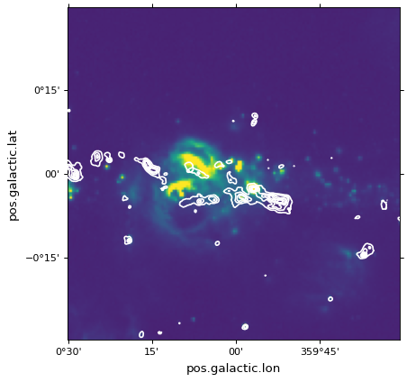
Contours#
Overplotting contours is also simple using the
get_transform() method. For contours,
get_transform() should be given the WCS of the
image to plot the contours for:
filename = get_pkg_data_filename('galactic_center/gc_bolocam_gps.fits')
hdu = fits.open(filename)[0]
ax.contour(hdu.data, transform=ax.get_transform(WCS(hdu.header)),
           levels=[1,2,3,4,5,6], colors='white')
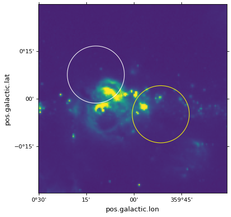
Spherical patches#
In the case where you are making a plot of a celestial image, and want to plot a circle that represents the area within a certain angle of a longitude/latitude,
the Circle patch is not appropriate, since it will result in a distorted shape (because longitude is not the same as the angle on the sky).
For this use case, you can instead use SphericalCircle, which takes a tuple of Quantity or a SkyCoord object as the input,
and a Quantity as the radius:
from astropy import units as u
from astropy.coordinates import SkyCoord
from astropy.visualization.wcsaxes import SphericalCircle


r = SphericalCircle((266.4 * u.deg, -29.1 * u.deg), 0.15 * u.degree,
                     edgecolor='yellow', facecolor='none',
                     transform=ax.get_transform('fk5'))

ax.add_patch(r)

#The following lines show the usage of a SkyCoord object as the input.
skycoord_object = SkyCoord(266.4 * u.deg, -28.7 * u.deg)
s = SphericalCircle(skycoord_object, 0.15 * u.degree,
                    edgecolor='white', facecolor='none',
                    transform=ax.get_transform('fk5'))

ax.add_patch(s)
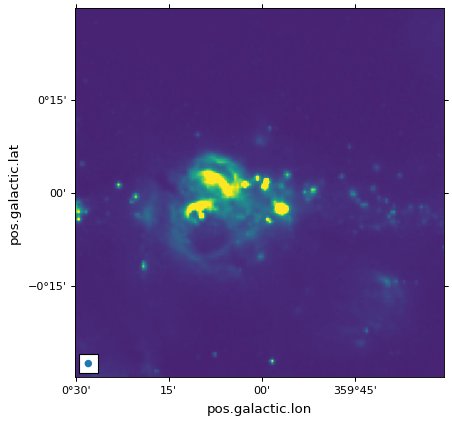
Beam shape and scale bar#
Adding an ellipse that represents the shape of the beam on a celestial
image can be done with the
add_beam() function:
from astropy import units as u
from astropy.visualization.wcsaxes import add_beam, add_scalebar

add_beam(ax, major=1.2 * u.arcmin, minor=1.2 * u.arcmin, angle=0, frame=True)
To add a segment that shows a physical scale, you can use the
add_scalebar() function:
# Compute the angle corresponding to 10 pc at the distance of the galactic center
gc_distance = 8.2 * u.kpc
scalebar_length = 10 * u.pc
scalebar_angle = (scalebar_length / gc_distance).to(
    u.deg, equivalencies=u.dimensionless_angles()
)

# Add a scale bar
add_scalebar(ax, scalebar_angle, label="10 pc", color="white")
