Creating color RGB images#
RGB images can be produced using matplotlib’s ability to make three-color images. In general, an RGB image is an MxNx3 array, where M is the y-dimension, N is the x-dimension, and the length-3 layer represents red, green, and blue, respectively. A fourth layer representing the alpha (opacity) value can be specified.
Matplotlib has several tools for manipulating these colors at
matplotlib.colors.
Astropy’s visualization tools can be used to change the stretch and scaling of the individual layers of the RGB image. Each layer must be on a scale of 0-1 for floats (or 0-255 for integers); values outside that range will be clipped.
RGB images using the Lupton et al (2004) scheme#
Lupton et al. (2004) describe an “optimal” algorithm for producing
red-green-blue composite images from three separate high-dynamic range arrays. This method
is implemented in make_lupton_rgb() as a convenience
wrapper function and an associated set of classes to provide alternate scalings.
The SDSS SkyServer color images were made using a variation on this technique.
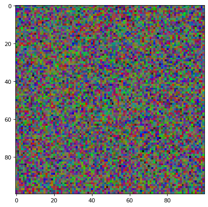
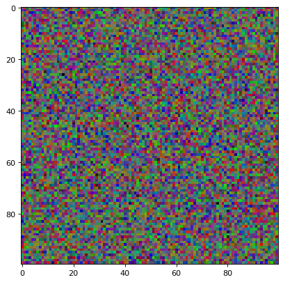
To generate a color PNG file with the default (arcsinh) scaling:
import numpy as np
import matplotlib.pyplot as plt
from astropy.visualization import make_lupton_rgb
rng = np.random.default_rng()
image_r = rng.random((100,100))
image_g = rng.random((100,100))
image_b = rng.random((100,100))
image = make_lupton_rgb(image_r, image_g, image_b, stretch=0.5)
fig, ax = plt.subplots()
ax.imshow(image)
This method requires that the three images be aligned and have the same pixel
scale and size. Changing the interval from the default of an instance of
ManualInterval() with vmin=0 (alternatively,
passing the keyword minimum) will change the black level. The parameters
stretch and Q will change how the values between black and white are
scaled.
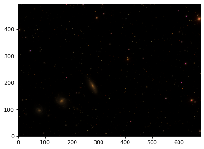
For a more in-depth example, download the g, r, i SDSS frames
(they will serve as the blue, green and red channels respectively) of
the area around the Hickson 88 group and try the example below and compare
it with Figure 1 of Lupton et al. (2004):
import matplotlib.pyplot as plt
from astropy.visualization import make_lupton_rgb
from astropy.io import fits
from astropy.utils.data import get_pkg_data_filename

# Read in the three images downloaded from here:
g_name = get_pkg_data_filename('visualization/reprojected_sdss_g.fits.bz2')
r_name = get_pkg_data_filename('visualization/reprojected_sdss_r.fits.bz2')
i_name = get_pkg_data_filename('visualization/reprojected_sdss_i.fits.bz2')
g = fits.getdata(g_name)
r = fits.getdata(r_name)
i = fits.getdata(i_name)

rgb_default = make_lupton_rgb(i, r, g, filename="ngc6976-default.jpeg")
fig, ax = plt.subplots()
ax.imshow(rgb_default, origin='lower')

The image above was generated with the default parameters. However using a different scaling, e.g Q=10, stretch=0.5, faint features of the galaxies show up. Compare with Fig. 1 of Lupton et al. (2004) or the SDSS Skyserver image.
rgb = make_lupton_rgb(i, r, g, Q=10, stretch=0.5, filename="ngc6976.jpeg")
fig, ax = plt.subplots()
ax.imshow(rgb, origin='lower')


RGB images using arbitrary stretching#
Numerous other methods for generating composite RGB images are possible. Alternative choices include using e.g., linear or logarithmic stretches, combined with optional data clipping and normalization (e.g., as often used in DS9 or other data viewers).
The image stretching and normalization methods for single images are
demonstrated in Image stretching and normalization.
These scaling are extended to the generation of RGB images using the
convenience function make_rgb(), which takes an
instance of a subclass of BaseStretch in
addition to either an instance of a subclass of
BaseInterval to specify the normalization,
or a length-3 array of such instances (to separately specify the per-filter
intervals).
By default, make_rgb() uses as linear
stretch (LinearStretch) and
a one-sided manual interval (ManualInterval,
with vmin=0). As with make_lupton_rgb(),
the three images mustbe aligned, with the same size and pixel scales.
Following the above example, we generate a composite RGB image using the
g, r, i SDSS frames around the Hickson 88 group,
now using a linear scaling.
import numpy as np
import matplotlib.pyplot as plt
from astropy.visualization import make_rgb, ManualInterval
from astropy.io import fits
from astropy.utils.data import get_pkg_data_filename

# Read in the three images downloaded from here:
g_name = get_pkg_data_filename('visualization/reprojected_sdss_g.fits.bz2')
r_name = get_pkg_data_filename('visualization/reprojected_sdss_r.fits.bz2')
i_name = get_pkg_data_filename('visualization/reprojected_sdss_i.fits.bz2')
g = fits.getdata(g_name)
r = fits.getdata(r_name)
i = fits.getdata(i_name)

# Use the maximum value of the 99.5% percentile over all three filters
# as the maximum value:
pctl = 99.5
maximum = 0.
for img in [i,r,g]:
    val = np.percentile(img,pctl)
    if val > maximum:
        maximum = val
rgb = make_rgb(i, r, g, interval=ManualInterval(vmin=0, vmax=maximum),
               filename="ngc6976-linear.jpeg")

fig, ax = plt.subplots()
ax.imshow(rgb, origin='lower')

For images with high dynamic range, logarithmic stretches with values calculated as
can be beneficial. In this case, the a stretch instance of
LogStretch is directly passed:
from astropy.visualization import LogStretch

# Use the maximum value of the 99.95% percentile over all three filters
# as the maximum value:
pctl = 99.95
maximum = 0.
for img in [i,r,g]:
    val = np.percentile(img,pctl)
    if val > maximum:
        maximum = val

rgb_log = make_rgb(i, r, g, interval=ManualInterval(vmin=0, vmax=maximum),
                   stretch=LogStretch(a=1000), filename="ngc6976-log.jpeg")

fig, ax = plt.subplots()
ax.imshow(rgb_log, origin='lower')


By specifying per-filter maximum values, it is possible to emphasize certain objects, such as the very reddest sources:
# Increase the red maximum to emphasize the very reddest sources:
intervals = 3 * [ManualInterval(vmin=0, vmax=maximum)]
intervals[0] = ManualInterval(vmin=0, vmax=30.)
rgb_log = make_rgb(i, r, g, interval=intervals, stretch=LogStretch(a=1000),
                   filename="ngc6976-log-alt.jpeg")

fig, ax = plt.subplots()
ax.imshow(rgb_log, origin='lower')


Other stretches, such as square root, can also be used:
from astropy.visualization import SqrtStretch

# Use the maximum value of the 99.8% percentile over all three filters
# as the maximum value:
pctl = 99.8
maximum = 0.
for img in [i,r,g]:
    val = np.percentile(img,pctl)
    if val > maximum:
        maximum = val

rgb_sqrt = make_rgb(i, r, g, interval=ManualInterval(vmin=0, vmax=maximum),
                    stretch=SqrtStretch(), filename="ngc6976-sqrt.jpeg")

fig, ax = plt.subplots()
ax.imshow(rgb_sqrt, origin='lower')


