Box Least Squares (BLS) Periodogram#
The “box least squares” (BLS) periodogram [1] is a statistical tool used for
detecting transiting exoplanets and eclipsing binaries in time series
photometric data. The main interface to this implementation is the
BoxLeastSquares class.
Mathematical Background#
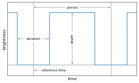
The BLS method finds transit candidates by modeling a transit as a periodic upside down top hat with four parameters: period, duration, depth, and a reference time. In this implementation, the reference time is chosen to be the mid-transit time of the first transit in the observational baseline. These parameters are shown in the following sketch:
Assuming that the uncertainties on the measured flux are known, independent, and Gaussian, the maximum likelihood in-transit flux can be computed as
where \(y_n\) are the brightness measurements, \(\sigma_n\) are the associated uncertainties, and both sums are computed over the in-transit data points.
Similarly, the maximum likelihood out-of-transit flux is
where these sums are over the out-of-transit observations. Using these results, the log likelihood of a transit model (maximized over depth) at a given period \(P\), duration \(\tau\), and reference time \(t_0\) is
This equation might be familiar because it is proportional to the “chi squared” \(\chi^2\) for this model and this is a direct consequence of our assumption of Gaussian uncertainties.
This \(\chi^2\) is called the “signal residue” by [1], so maximizing the log likelihood over duration and reference time is equivalent to computing the box least squares spectrum from [1].
In practice, this is achieved by finding the maximum likelihood model over a
grid in duration and reference time as specified by the durations and
oversample parameters for the
power method.
Behind the scenes, this implementation minimizes the number of required calculations by pre-binning the observations onto a fine grid following [1] and [2].
Basic Usage#
The transit periodogram takes as input time series observations where the
timestamps t and the observations y (usually brightness) are stored as
numpy arrays or Quantity objects. If known, error
bars dy can also optionally be provided.
Example#
To evaluate the periodogram for a simulated data set:
>>> import numpy as np
>>> import astropy.units as u
>>> from astropy.timeseries import BoxLeastSquares
>>> rng = np.random.default_rng(42)
>>> t = rng.uniform(0, 20, 2000)
>>> y = np.ones_like(t) - 0.1*((t%3)<0.2) + 0.01*rng.standard_normal(len(t))
>>> model = BoxLeastSquares(t * u.day, y, dy=0.01)
>>> periodogram = model.autopower(0.2)
The output of the astropy.timeseries.BoxLeastSquares.autopower method
is a BoxLeastSquaresResults object with several
useful attributes, the most useful of which are generally the period and
power attributes.
This result can be plotted using matplotlib:
>>> import matplotlib.pyplot as plt
>>> fig, ax = plt.subplots()
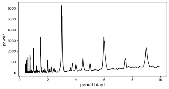
>>> ax.plot(periodogram.period, periodogram.power)
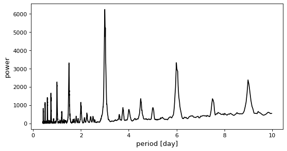
In this figure, you can see the peak at the correct period of three days.
Objectives#
By default, the power method computes the
log likelihood of the model fit and maximizes over reference time and duration.
It is also possible to use the signal-to-noise ratio with which the transit
depth is measured as an objective function.
Example#
To compute the log likelihood of the model fit, call
power or
autopower with objective='snr' as
follows:
>>> model = BoxLeastSquares(t * u.day, y, dy=0.01)
>>> periodogram = model.autopower(0.2, objective="snr")
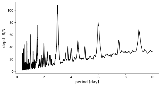
This objective will generally produce a periodogram that is qualitatively similar to the log likelihood spectrum, but it has been used to improve the reliability of transit search in the presence of correlated noise.
Period Grid#
The transit periodogram is always computed on a grid of periods and the results
can be sensitive to the sampling. As discussed in [1], the performance of the
transit periodogram method is more sensitive to the period grid than the
LombScargle periodogram.
This implementation of the transit periodogram includes a conservative heuristic
for estimating the required period grid that is used by the
autoperiod and
autopower methods and the details of this
method are given in the API documentation for
autoperiod.
Example#
It is possible to provide a specific period grid as follows:
>>> model = BoxLeastSquares(t * u.day, y, dy=0.01)
>>> periods = np.linspace(2.5, 3.5, 1000) * u.day
>>> periodogram = model.power(periods, 0.2)
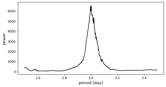
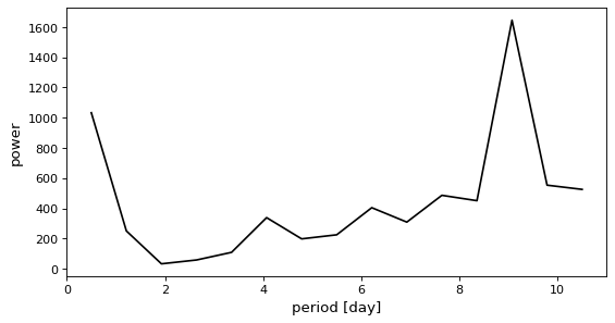
However, if the period grid is too coarse, the correct period might be missed.
>>> model = BoxLeastSquares(t * u.day, y, dy=0.01)
>>> periods = np.linspace(0.5, 10.5, 15) * u.day
>>> periodogram = model.power(periods, 0.2)
Peak Statistics#
To help in the transit vetting process and to debug problems with candidate
peaks, the compute_stats method can be
used to calculate several statistics of a candidate transit.
Many of these statistics are based on the VARTOOLS package described in [2]. This will often be used as follows to compute stats for the maximum point in the periodogram:
>>> model = BoxLeastSquares(t * u.day, y, dy=0.01)
>>> periodogram = model.autopower(0.2)
>>> max_power = np.argmax(periodogram.power)
>>> stats = model.compute_stats(periodogram.period[max_power],
...                             periodogram.duration[max_power],
...                             periodogram.transit_time[max_power])
This calculates a dictionary with statistics about this candidate.
Each entry in this dictionary is described in the documentation for
compute_stats.