Fitting Models to Data#
This module provides wrappers, called Fitters, around some Numpy and Scipy
fitting functions. All Fitters can be called as functions. They take an
instance of FittableModel as input and modify its
parameters attribute. The idea is to make this extensible and allow
users to easily add other fitters.
Linear fitting is done using Numpy’s numpy.linalg.lstsq function. There are
currently non-linear fitters which use scipy.optimize.leastsq,
scipy.optimize.least_squares, and scipy.optimize.fmin_slsqp.
The rules for passing input to fitters are:
Non-linear fitters currently work only with single models (not model sets).
The linear fitter can fit a single input to multiple model sets creating multiple fitted models. This may require specifying the
model_set_axisargument just as used when evaluating models; this may be required for the fitter to know how to broadcast the input data.The
LinearLSQFittercurrently works only with simple (not compound) models.The current fitters work only with models that have a single output (including bivariate functions such as
Chebyshev2Dbut not compound models that mapx, y -> x', y').The units of the fitting data and the model parameters are stripped before fitting so that the underlying
scipymethods can handle this data. One should be aware of this when fitting data with units as unit conversions will only be performed initially. These conversions will be performed using theequivalenciesargument to the fitter combined with themodel.input_units_equivalenciesattribute of the model being fit.
Note
In general, non-linear fitters do not support fitting to data which contains
non-finite values: NaN, Inf, or -Inf. This is a limitation of the
underlying scipy library. As a consequence, an error will be raised whenever
any non-finite value is present in the data to be fitted. To avoid this error
users should “filter” the non-finite values from their data, for example
when fitting a model, with a fitter using data containing non-finite
values one can “filter” these problems as follows for the 1D case:
# Filter non-finite values from data
mask = np.isfinite(data)
# Fit model to filtered data
model = fitter(model, x[mask], data[mask])
or for the 2D case:
# Filter non-finite values from data
mask = np.isfinite(data)
# Fit model to filtered data
model = fitter(model, x[mask], y[mask], data[mask])
Notes on non-linear fitting#
There are several non-linear fitters, which rely on several different optimization algorithms now. Choice of algorithm is problem dependent. The main non-linear fitters are:
LevMarLSQFitter, which uses the Levenberg-Marquardt algorithm via the scipy legacy functionscipy.optimize.leastsq. This fitter supports parameter bounds via an unsophisticated min/max condition which can cause parameters to “stick” to one of the bounds if during the fitting process the parameter gets close to the bound during some of the intermediate fitting operations.TRFLSQFitter, which uses the Trust Region Reflective (TRF) algorithm that is particularly suitable for large sparse problems with bounds, seescipy.optimize.least_squaresfor more details. Note that this fitter supports parameter bounds in a sophisticated fashion which prevents fitting from “sticking” to one of the bounds provided. This fitter can be switched over to using the min/max bound method by settinguse_min_max_bounds=Falsewhen initializing the fitter. This is the recommended algorithm by scipy.DogBoxLSQFitter, which uses the dogleg algorithm with rectangular trust regions, typical use case is small problems with bounds. Not recommended for problems with rank-deficient Jacobian, seescipy.optimize.least_squaresfor more details. This fitter supports bounds in the same fashion thatTRFLSQFitterdoes.LMLSQFitter, which uses the Levenberg-Marquardt (LM) algorithm as implemented byscipy.optimize.least_squares. Does not handle bounds and/or sparse Jacobians. Usually the most efficient method for small unconstrained problems. If a Levenberg-Marquardt algorithm is desired for your problem, it is now recommended that you use this fitter instead ofLevMarLSQFitteras it makes use of the recommended version of this algorithm in scipy.
Simple 1-D model fitting#
In this section, we look at a simple example of fitting a Gaussian to a
simulated dataset. We use the Gaussian1D
and Trapezoid1D models and the
LevMarLSQFitter fitter to fit the data:
import numpy as np
import matplotlib.pyplot as plt
from astropy.modeling import models, fitting

# Generate fake data
rng = np.random.default_rng(0)
x = np.linspace(-5., 5., 200)
y = 3 * np.exp(-0.5 * (x - 1.3)**2 / 0.8**2)
y += rng.normal(0., 0.2, x.shape)

# Fit the data using a box model.
# Bounds are not really needed but included here to demonstrate usage.
t_init = models.Trapezoid1D(amplitude=1., x_0=0., width=1., slope=0.5,
                            bounds={"x_0": (-5., 5.)})
fit_t = fitting.LevMarLSQFitter()
t = fit_t(t_init, x, y, maxiter=200)

# Fit the data using a Gaussian
g_init = models.Gaussian1D(amplitude=1., mean=0, stddev=1.)
fit_g = fitting.LevMarLSQFitter()
g = fit_g(g_init, x, y)

# Plot the data with the best-fit model
plt.figure(figsize=(8,5))
plt.plot(x, y, 'ko')
plt.plot(x, t(x), label='Trapezoid')
plt.plot(x, g(x), label='Gaussian')
plt.xlabel('Position')
plt.ylabel('Flux')
plt.legend(loc=2)
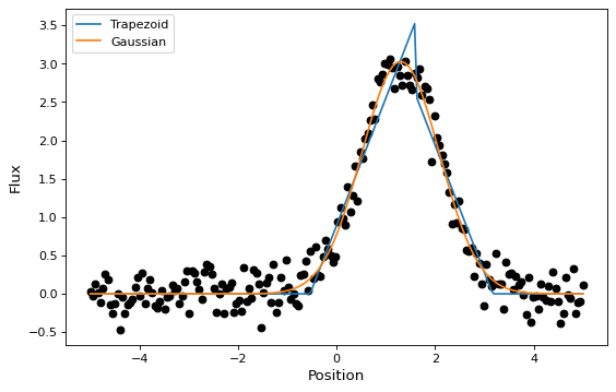
As shown above, once instantiated, the fitter class can be used as a function
that takes the initial model (t_init or g_init) and the data values
(x and y), and returns a fitted model (t or g).
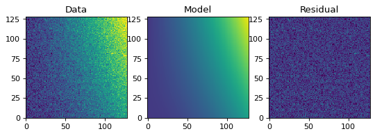
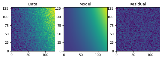
Simple 2-D model fitting#
Similarly to the 1-D example, we can create a simulated 2-D data dataset, and fit a polynomial model to it. This could be used for example to fit the background in an image.
import warnings
import numpy as np
import matplotlib.pyplot as plt
from astropy.modeling import models, fitting
from astropy.utils.exceptions import AstropyUserWarning

# Generate fake data
rng = np.random.default_rng(0)
y, x = np.mgrid[:128, :128]
z = 2. * x ** 2 - 0.5 * x ** 2 + 1.5 * x * y - 1.
z += rng.normal(0., 0.1, z.shape) * 50000.

# Fit the data using astropy.modeling
p_init = models.Polynomial2D(degree=2)
fit_p = fitting.LevMarLSQFitter()

with warnings.catch_warnings():
    # Ignore model linearity warning from the fitter
    warnings.filterwarnings('ignore', message='Model is linear in parameters',
                            category=AstropyUserWarning)
    p = fit_p(p_init, x, y, z)

# Plot the data with the best-fit model
plt.figure(figsize=(8, 2.5))
plt.subplot(1, 3, 1)
plt.imshow(z, origin='lower', interpolation='nearest', vmin=-1e4, vmax=5e4)
plt.title("Data")
plt.subplot(1, 3, 2)
plt.imshow(p(x, y), origin='lower', interpolation='nearest', vmin=-1e4,
           vmax=5e4)
plt.title("Model")
plt.subplot(1, 3, 3)
plt.imshow(z - p(x, y), origin='lower', interpolation='nearest', vmin=-1e4,
           vmax=5e4)
plt.title("Residual")