
Working with Velocities in Astropy Coordinates#
Using Velocities with SkyCoord#
The best way to start getting a coordinate object with velocities is to use the
SkyCoord interface.
Examples#
A SkyCoord to represent a star with a measured radial velocity but unknown
proper motion and distance could be created as:
>>> from astropy.coordinates import SkyCoord
>>> import astropy.units as u
>>> sc = SkyCoord(1*u.deg, 2*u.deg, radial_velocity=20*u.km/u.s)
>>> sc
<SkyCoord (ICRS): (ra, dec) in deg
    (1., 2.)
 (radial_velocity) in km / s
    (20.,)>
>>> sc.radial_velocity
<Quantity 20.0 km / s>
SkyCoord objects created in this manner follow all of the same transformation
rules and will correctly update their velocities when transformed to other
frames. For example, to determine proper motions in Galactic coordinates for
a star with proper motions measured in ICRS:
>>> sc = SkyCoord(1*u.deg, 2*u.deg, pm_ra_cosdec=.2*u.mas/u.yr, pm_dec=.1*u.mas/u.yr)
>>> sc.galactic
<SkyCoord (Galactic): (l, b) in deg
  ( 99.63785528, -58.70969293)
(pm_l_cosb, pm_b) in mas / yr
  ( 0.22240398,  0.02316181)>
For more details on valid operations and limitations of velocity support in
astropy.coordinates (particularly the current accuracy limitations), see the more detailed
discussions below of velocity support in the lower-level frame objects. All
these same rules apply for SkyCoord objects, as they are built directly on top
of the frame classes’ velocity functionality detailed here.
Creating Frame Objects with Velocity Data#
The coordinate frame classes support storing and transforming velocity data
(alongside the positional coordinate data). Similar to the positional data that
use the Representation classes to abstract away the particular
representation and allow re-representing from (e.g., Cartesian to Spherical),
the velocity data makes use of Differential classes to do the
same. (For more information about the differential classes, see
Differentials and Derivatives of Representations.) Also like the positional data, the
names of the differential (velocity) components depend on the particular
coordinate frame.
Most frames expect velocity data in the form of two proper motion components
and/or a radial velocity because the default differential for most frames is the
SphericalCosLatDifferential class. When supported, the
proper motion components all begin with pm_ and, by default, the
longitudinal component is expected to already include the cos(latitude)
term. For example, the proper motion components for the ICRS frame are
(pm_ra_cosdec, pm_dec).
Examples#
To create frame objects with velocity data in the form of proper motion components:
>>> from astropy.coordinates import ICRS
>>> ICRS(ra=8.67*u.degree, dec=53.09*u.degree,
...      pm_ra_cosdec=4.8*u.mas/u.yr, pm_dec=-15.16*u.mas/u.yr)
<ICRS Coordinate: (ra, dec) in deg
    (8.67, 53.09)
 (pm_ra_cosdec, pm_dec) in mas / yr
    (4.8, -15.16)>
>>> ICRS(ra=8.67*u.degree, dec=53.09*u.degree,
...      pm_ra_cosdec=4.8*u.mas/u.yr, pm_dec=-15.16*u.mas/u.yr,
...      radial_velocity=23.42*u.km/u.s)
<ICRS Coordinate: (ra, dec) in deg
    (8.67, 53.09)
 (pm_ra_cosdec, pm_dec, radial_velocity) in (mas / yr, mas / yr, km / s)
    (4.8, -15.16, 23.42)>
For proper motion components in the Galactic frame, the names track the
longitude and latitude names:
>>> from astropy.coordinates import Galactic
>>> Galactic(l=11.23*u.degree, b=58.13*u.degree,
...          pm_l_cosb=21.34*u.mas/u.yr, pm_b=-55.89*u.mas/u.yr)
<Galactic Coordinate: (l, b) in deg
    (11.23, 58.13)
 (pm_l_cosb, pm_b) in mas / yr
    (21.34, -55.89)>
Like the positional data, velocity data must be passed in as
Quantity objects.
The expected differential class can be changed to control the argument names
that the frame expects. By default the proper motion components are expected to
contain the cos(latitude), but this can be changed by specifying the
SphericalDifferential class (instead of the default
SphericalCosLatDifferential):
>>> from astropy.coordinates import SphericalDifferential
>>> Galactic(l=11.23*u.degree, b=58.13*u.degree,
...          pm_l=21.34*u.mas/u.yr, pm_b=-55.89*u.mas/u.yr,
...          differential_type=SphericalDifferential)
<Galactic Coordinate: (l, b) in deg
    (11.23, 58.13)
 (pm_l, pm_b) in mas / yr
    (21.34, -55.89)>
This works in parallel to specifying the expected representation class, as long as the differential class is compatible with the representation. For example, to specify all coordinate and velocity components in Cartesian:
>>> from astropy.coordinates import (CartesianRepresentation,
...                                  CartesianDifferential)
>>> Galactic(u=103*u.pc, v=-11*u.pc, w=93.*u.pc,
...          U=31*u.km/u.s, V=-10*u.km/u.s, W=75*u.km/u.s,
...          representation_type=CartesianRepresentation,
...          differential_type=CartesianDifferential)
<Galactic Coordinate: (u, v, w) in pc
    (103., -11., 93.)
 (U, V, W) in km / s
    (31., -10., 75.)>
Note that the Galactic frame has special, standard names for Cartesian
position and velocity components. For other frames, these are just x,y,z and
v_x,v_y,v_z:
>>> ICRS(x=103*u.pc, y=-11*u.pc, z=93.*u.pc,
...      v_x=31*u.km/u.s, v_y=-10*u.km/u.s, v_z=75*u.km/u.s,
...      representation_type=CartesianRepresentation,
...      differential_type=CartesianDifferential)
<ICRS Coordinate: (x, y, z) in pc
    (103., -11., 93.)
 (v_x, v_y, v_z) in km / s
    (31., -10., 75.)>
For any frame with velocity data with any representation, there are also shorthands that provide easier access to the underlying velocity data in commonly needed formats. With any frame object with 3D velocity data, the 3D Cartesian velocity can be accessed with:
>>> icrs = ICRS(ra=8.67*u.degree, dec=53.09*u.degree,
...             distance=171*u.pc,
...             pm_ra_cosdec=4.8*u.mas/u.yr, pm_dec=-15.16*u.mas/u.yr,
...             radial_velocity=23.42*u.km/u.s)
>>> icrs.velocity
<CartesianDifferential (d_x, d_y, d_z) in km / s
    ( 23.03160789,  7.44794505,  11.34587732)>
There are also shorthands for retrieving a single Quantity
object that contains the two-dimensional proper motion data, and for retrieving
the radial (line-of-sight) velocity:
>>> icrs.proper_motion
<Quantity [  4.8 ,-15.16] mas / yr>
>>> icrs.radial_velocity
<Quantity 23.42 km / s>
Adding Velocities to Existing Frame Objects#
Another use case similar to the above comes up when you have an existing frame
object (or SkyCoord) and want an object with the same position but with
velocities added. The most conceptually direct way to do this is to
use the differential objects along with
realize_frame.
Examples#
The following snippet accomplishes a well-defined case where the desired
velocities are known in the Cartesian representation. To add the velocities to
the existing frame using
realize_frame:
>>> icrs = ICRS(1*u.deg, 2*u.deg, distance=3*u.kpc)
>>> icrs
<ICRS Coordinate: (ra, dec, distance) in (deg, deg, kpc)
    (1., 2., 3.)>
>>> vel_to_add = CartesianDifferential(4*u.km/u.s, 5*u.km/u.s, 6*u.km/u.s)
>>> newdata = icrs.data.to_cartesian().with_differentials(vel_to_add)
>>> icrs.realize_frame(newdata)
<ICRS Coordinate: (ra, dec, distance) in (deg, deg, kpc)
    (1., 2., 3.)
 (pm_ra_cosdec, pm_dec, radial_velocity) in (mas / yr, mas / yr, km / s)
    (0.34662023, 0.41161335, 4.29356031)>
A similar mechanism can also be used to add velocities even if full 3D coordinates are not available (e.g., for a radial velocity observation of an object where the distance is unknown). However, it requires a slightly different way of specifying the differentials because of the lack of explicit unit information:
>>> from astropy.coordinates import RadialDifferential
>>> icrs_no_distance = ICRS(1*u.deg, 2*u.deg)
>>> icrs_no_distance
<ICRS Coordinate: (ra, dec) in deg
    (1., 2.)>
>>> rv_to_add = RadialDifferential(500*u.km/u.s)
>>> data_with_rv = icrs_no_distance.data.with_differentials({'s':rv_to_add})
>>> icrs_no_distance.realize_frame(data_with_rv)
<ICRS Coordinate: (ra, dec) in deg
    (1., 2.)
 (radial_velocity) in km / s
    (500.,)>
Which we can see yields an object identical to what you get when you specify a radial velocity when you create the object:
>>> ICRS(1*u.deg, 2*u.deg, radial_velocity=500*u.km/u.s)
<ICRS Coordinate: (ra, dec) in deg
    (1., 2.)
 (radial_velocity) in km / s
    (500.,)>
Transforming Frames with Velocities#
Transforming coordinate frame instances that contain velocity data to a different frame (which may involve both position and velocity transformations) is done exactly the same way as transforming position-only frame instances.
Example#
To transform a coordinate frame that contains velocity data:
>>> from astropy.coordinates import Galactic
>>> icrs = ICRS(ra=8.67*u.degree, dec=53.09*u.degree,
...             pm_ra_cosdec=4.8*u.mas/u.yr, pm_dec=-15.16*u.mas/u.yr)
>>> icrs.transform_to(Galactic())
<Galactic Coordinate: (l, b) in deg
    (120.38084191, -9.69872044)
 (pm_l_cosb, pm_b) in mas / yr
    (3.78957965, -15.44359693)>
However, the details of how the velocity components are transformed depends on
the particular set of transforms required to get from the starting frame to the
desired frame (i.e., the path taken through the frame transform graph). If all
frames in the chain of transformations are transformed to each other via
BaseAffineTransform subclasses (i.e., are matrix
transformations or affine transformations), then the transformations can be
applied explicitly to the velocity data. If this is not the case, the velocity
transformation is computed numerically by finite-differencing the positional
transformation. See the subsections below for more details about these two
methods.
Affine Transformations#
Frame transformations that involve a rotation and/or an origin shift and/or
a velocity offset are implemented as affine transformations using the
BaseAffineTransform subclasses:
StaticMatrixTransform,
DynamicMatrixTransform, and
AffineTransform.
Matrix-only transformations (e.g., rotations such as
ICRS to Galactic) can be performed
on proper-motion-only data or full-space, 3D velocities.
Examples#
To perform a matrix-only transformation:
>>> icrs = ICRS(ra=8.67*u.degree, dec=53.09*u.degree,
...             pm_ra_cosdec=4.8*u.mas/u.yr, pm_dec=-15.16*u.mas/u.yr,
...             radial_velocity=23.42*u.km/u.s)
>>> icrs.transform_to(Galactic())
<Galactic Coordinate: (l, b) in deg
    (120.38084191, -9.69872044)
 (pm_l_cosb, pm_b, radial_velocity) in (mas / yr, mas / yr, km / s)
    (3.78957965, -15.44359693, 23.42)>
The same rotation matrix is applied to both the position vector and the velocity
vector. Any transformation that involves a velocity offset requires all 3D
velocity components (which typically require specifying a distance as well),
for example, ICRS to LSR:
>>> from astropy.coordinates import LSR
>>> icrs = ICRS(ra=8.67*u.degree, dec=53.09*u.degree,
...             distance=117*u.pc,
...             pm_ra_cosdec=4.8*u.mas/u.yr, pm_dec=-15.16*u.mas/u.yr,
...             radial_velocity=23.42*u.km/u.s)
>>> icrs.transform_to(LSR())
<LSR Coordinate (v_bary=(11.1, 12.24, 7.25) km / s): (ra, dec, distance) in (deg, deg, pc)
    (8.67, 53.09, 117.)
 (pm_ra_cosdec, pm_dec, radial_velocity) in (mas / yr, mas / yr, km / s)
    (-24.51315607, -2.67935501, 27.07339176)>
Finite Difference Transformations#
Some frame transformations cannot be expressed as affine transformations.
For example, transformations from the AltAz frame can
include an atmospheric dispersion correction, which is inherently nonlinear.
Additionally, some frames are more conveniently implemented as functions, even
if they can be cast as affine transformations. For these frames, a finite
difference approach to transforming velocities is available. Note that this
approach is implemented such that user-defined frames can use it in
the same manner (i.e., by defining a transformation of the
FunctionTransformWithFiniteDifference type).
This finite difference approach actually combines two separate (but important) elements of the transformation:
Transformation of the direction of the velocity vector that already exists in the starting frame. That is, a frame transformation sometimes involves reorienting the coordinate frame (e.g., rotation), and the velocity vector in the new frame must account for this. The finite difference approach models this by moving the position of the starting frame along the velocity vector, and computing this offset in the target frame.
The “induced” velocity due to motion of the frame itself. For example, shifting from a frame centered at the solar system barycenter to one centered on the Earth includes a velocity component due entirely to the Earth’s motion around the barycenter. This is accounted for by computing the location of the starting frame in the target frame at slightly different times, and computing the difference between those. Note that this step depends on assuming that a particular frame attribute represents a “time” of relevance for the induced velocity. By convention this is typically the
obstimeframe attribute, although it is an option that can be set when defining a finite difference transformation function.
Example#
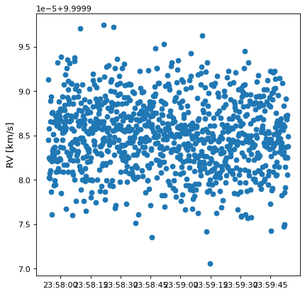
It is important to recognize that the finite difference transformations have inherent limits set by the finite difference algorithm and machine precision. To illustrate this problem, consider the AltAz to GCRS (i.e., geocentric) transformation. Let us try to compute the radial velocity in the GCRS frame for something observed from the Earth at a distance of 100 AU with a radial velocity of 10 km/s:
import numpy as np
from matplotlib import pyplot as plt

from astropy import units as u
from astropy.time import Time
from astropy.coordinates import EarthLocation, AltAz, GCRS

time = Time('J2010') + np.linspace(-1,1,1000)*u.min
location = EarthLocation(lon=0*u.deg, lat=45*u.deg)
aa = AltAz(alt=[45]*1000*u.deg, az=90*u.deg, distance=100*u.au,
           radial_velocity=[10]*1000*u.km/u.s,
           location=location, obstime=time)
gcrs = aa.transform_to(GCRS(obstime=time))
plt.plot_date(time.plot_date, gcrs.radial_velocity.to(u.km/u.s))
plt.ylabel('RV [km/s]')

This seems plausible: the radial velocity should indeed be very close to 10 km/s because the frame does not involve a velocity shift.
Now let us consider 100 kiloparsecs as the distance. In this case we expect the same: the radial velocity should be essentially the same in both frames:
time = Time('J2010') + np.linspace(-1,1,1000)*u.min
location = EarthLocation(lon=0*u.deg, lat=45*u.deg)
aa = AltAz(alt=[45]*1000*u.deg, az=90*u.deg, distance=100*u.kpc,
           radial_velocity=[10]*1000*u.km/u.s,
           location=location, obstime=time)
gcrs = aa.transform_to(GCRS(obstime=time))
plt.plot_date(time.plot_date, gcrs.radial_velocity.to(u.km/u.s))
plt.ylabel('RV [km/s]')
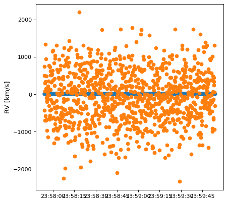
But this result is nonsense, with values from -1000 to 1000 km/s instead of the ~10 km/s we expected. The root of the problem here is that the machine precision is not sufficient to compute differences on the order of kilometers over distances on the order of kiloparsecs. Hence, the straightforward finite difference method will not work for this use case with the default values.
It is possible to override the timestep over which the finite difference occurs. For example:
>>> from astropy.coordinates import frame_transform_graph, AltAz, CIRS
>>> trans = frame_transform_graph.get_transform(AltAz, CIRS).transforms[0]
>>> trans.finite_difference_dt = 1 * u.year
>>> gcrs = aa.transform_to(GCRS(obstime=time))
>>> trans.finite_difference_dt = 1 * u.second  # return to default
In the above example, there is exactly one transformation step from
AltAz to GCRS. In general, there
may be more than one step between two frames, or the single step may perform
other transformations internally. One can use the context manager
impose_finite_difference_dt() for the
transformation graph to override finite_difference_dt for all
finite-difference transformations on the graph:
>>> from astropy.coordinates import frame_transform_graph
>>> with frame_transform_graph.impose_finite_difference_dt(1 * u.year):
...     gcrs = aa.transform_to(GCRS(obstime=time))
But beware that this will not help in cases like the above, where the relevant timescales for the velocities are seconds. (The velocity of the Earth relative to a particular direction changes dramatically over the course of one year.)
Future versions of Astropy will improve on this algorithm to make the results more numerically stable and practical for use in these (not unusual) use cases.
Radial Velocity Corrections#
Separately from the above, Astropy supports computing barycentric or
heliocentric radial velocity corrections. While in the future this may
be a high-level convenience function using the framework described above, the
current implementation is independent to ensure sufficient accuracy (see
Radial Velocity Corrections and the
radial_velocity_correction API docs for
details).
Example#
This example demonstrates how to compute this correction if observing some object at a known RA and Dec from the Keck observatory at a particular time. If a precision of around 3 m/s is sufficient, the computed correction can then be added to any observed radial velocity to determine the final heliocentric radial velocity:
>>> from astropy.time import Time
>>> from astropy.coordinates import SkyCoord, EarthLocation
>>> # keck = EarthLocation.of_site('Keck')  # the easiest way... but requires internet
>>> keck = EarthLocation.from_geodetic(lat=19.8283*u.deg, lon=-155.4783*u.deg, height=4160*u.m)
>>> sc = SkyCoord(ra=4.88375*u.deg, dec=35.0436389*u.deg)
>>> barycorr = sc.radial_velocity_correction(obstime=Time('2016-6-4'), location=keck)
>>> barycorr.to(u.km/u.s)
<Quantity 20.077135 km / s>
>>> heliocorr = sc.radial_velocity_correction('heliocentric', obstime=Time('2016-6-4'), location=keck)
>>> heliocorr.to(u.km/u.s)
<Quantity 20.070039 km / s>
Note that there are a few different ways to specify the options for the
correction (e.g., the location, observation time, etc.). See the
radial_velocity_correction docs for more
information.
Precision of radial_velocity_correction#
The correction computed by radial_velocity_correction
uses the optical approximation \(v = zc\) (see Spectral (Doppler) Equivalencies
for details). The correction can be added to any observed radial velocity
to provide a correction that is accurate to a level of approximately 3 m/s.
If you need more precise corrections, there are a number of subtleties of
which you must be aware.
The first is that you should always use a barycentric correction, as the
barycenter is a fixed point where gravity is constant. Since the heliocenter
does not satisfy these conditions, corrections to the heliocenter are only
suitable for low precision work. As a result, and to increase speed, the
heliocentric correction in
radial_velocity_correction does not include
effects such as the gravitational redshift due to the potential at the Earth’s
surface. For these reasons, the barycentric correction in
radial_velocity_correction should always
be used for high precision work.
Other considerations necessary for radial velocity corrections at the cm/s level are outlined in Wright & Eastman (2014). Most important is that the barycentric correction is, strictly speaking, multiplicative, so that you should apply it as:
Where \(v_t\) is the true radial velocity, \(v_m\) is the measured
radial velocity and \(v_b\) is the barycentric correction returned by
radial_velocity_correction. Failure to apply
the barycentric correction in this way leads to errors of order 3 m/s.
The barycentric correction in radial_velocity_correction is consistent
with the IDL implementation of
the Wright & Eastmann (2014) paper to a level of 10 mm/s for a source at
infinite distance. We do not include the Shapiro delay nor the light
travel time correction from equation 28 of that paper. The neglected terms
are not important unless you require accuracies of better than 1 cm/s.
If you do require that precision, see Wright & Eastmann (2014).