Creating color RGB images#
RGB images can be produced using matplotlib’s ability to make three-color images. In general, an RGB image is an MxNx3 array, where M is the y-dimension, N is the x-dimension, and the length-3 layer represents red, green, and blue, respectively. A fourth layer representing the alpha (opacity) value can be specified.
Matplotlib has several tools for manipulating these colors at
matplotlib.colors.
Astropy’s visualization tools can be used to change the stretch and scaling of the individual layers of the RGB image. Each layer must be on a scale of 0-1 for floats (or 0-255 for integers); values outside that range will be clipped.
Creating color RGB images using the Lupton et al (2004) scheme#
Lupton et al. (2004) describe an “optimal” algorithm for producing red-green-
blue composite images from three separate high-dynamic range arrays. This method
is implemented in make_lupton_rgb as a convenience
wrapper function and an associated set of classes to provide alternate scalings.
The SDSS SkyServer color images were made using a variation on this technique.
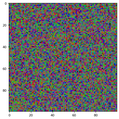
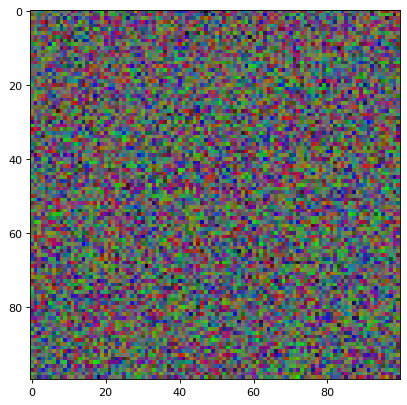
To generate a color PNG file with the default (arcsinh) scaling:
import numpy as np
import matplotlib.pyplot as plt
from astropy.visualization import make_lupton_rgb
rng = np.random.default_rng()
image_r = rng.random((100,100))
image_g = rng.random((100,100))
image_b = rng.random((100,100))
image = make_lupton_rgb(image_r, image_g, image_b, stretch=0.5)
plt.imshow(image)
This method requires that the three images be aligned and have the same pixel
scale and size. Changing minimum will change the black level, while
stretch and Q will change how the values between black and white are
scaled.
For a more in-depth example, download the g, r, i SDSS frames
(they will serve as the blue, green and red channels respectively) of
the area around the Hickson 88 group and try the example below and compare
it with Figure 1 of Lupton et al. (2004):
import matplotlib.pyplot as plt
from astropy.visualization import make_lupton_rgb
from astropy.io import fits
from astropy.utils.data import get_pkg_data_filename

# Read in the three images downloaded from here:
g_name = get_pkg_data_filename('visualization/reprojected_sdss_g.fits.bz2')
r_name = get_pkg_data_filename('visualization/reprojected_sdss_r.fits.bz2')
i_name = get_pkg_data_filename('visualization/reprojected_sdss_i.fits.bz2')
g = fits.open(g_name)[0].data
r = fits.open(r_name)[0].data
i = fits.open(i_name)[0].data

rgb_default = make_lupton_rgb(i, r, g, filename="ngc6976-default.jpeg")
plt.imshow(rgb_default, origin='lower')
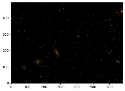
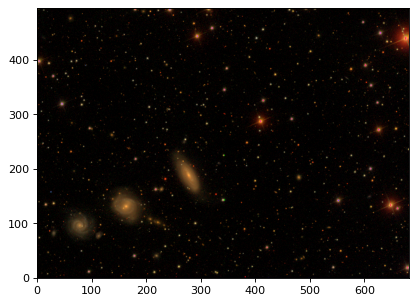
The image above was generated with the default parameters. However using a different scaling, e.g Q=10, stretch=0.5, faint features of the galaxies show up. Compare with Fig. 1 of Lupton et al. (2004) or the SDSS Skyserver image.
rgb = make_lupton_rgb(i, r, g, Q=10, stretch=0.5, filename="ngc6976.jpeg")
plt.imshow(rgb, origin='lower')