
Astronomical Coordinate Systems (astropy.coordinates)#
Introduction#
The coordinates package provides classes for representing a variety
of celestial/spatial coordinates and their velocity components, as well as tools
for converting between common coordinate systems in a uniform way.
Getting Started#
The best way to start using coordinates is to use the SkyCoord
class. SkyCoord objects are instantiated by passing in positions (and
optional velocities) with specified units and a coordinate frame. Sky positions
are commonly passed in as Quantity objects and the frame is
specified with the string name.
To create a SkyCoord object to represent an ICRS (Right ascension [RA],
Declination [Dec]) sky position:
>>> from astropy import units as u
>>> from astropy.coordinates import SkyCoord
>>> c = SkyCoord(ra=10.625*u.degree, dec=41.2*u.degree, frame='icrs')
The initializer for SkyCoord is very flexible and supports inputs provided in
a number of convenient formats. The following ways of initializing a coordinate
are all equivalent to the above:
>>> c = SkyCoord(10.625, 41.2, frame='icrs', unit='deg')
>>> c = SkyCoord('00h42m30s', '+41d12m00s', frame='icrs')
>>> c = SkyCoord('00h42.5m', '+41d12m')
>>> c = SkyCoord('00 42 30 +41 12 00', unit=(u.hourangle, u.deg))
>>> c = SkyCoord('00:42.5 +41:12', unit=(u.hourangle, u.deg))
>>> c
<SkyCoord (ICRS): (ra, dec) in deg
    (10.625, 41.2)>
The examples above illustrate a few rules to follow when creating a coordinate object:
Coordinate values can be provided either as unnamed positional arguments or via keyword arguments like
raanddec, orlandb(depending on the frame).The coordinate
framekeyword is optional because it defaults toICRS.Angle units must be specified for all components, either by passing in a
Quantityobject (e.g.,10.5*u.degree), by including them in the value (e.g.,'+41d12m00s'), or via theunitkeyword.
SkyCoord and all other coordinates objects also support
array coordinates. These work in the same way as single-value coordinates, but
they store multiple coordinates in a single object. When you are going
to apply the same operation to many different coordinates (say, from a
catalog), this is a better choice than a list of SkyCoord objects,
because it will be much faster than applying the operation to each
SkyCoord in a for loop. Like the underlying ndarray instances
that contain the data, SkyCoord objects can be sliced, reshaped, etc.,
and can be used with functions like numpy.moveaxis, etc., that affect the
shape:
>>> import numpy as np
>>> c = SkyCoord(ra=[10, 11, 12, 13]*u.degree, dec=[41, -5, 42, 0]*u.degree)
>>> c
<SkyCoord (ICRS): (ra, dec) in deg
    [(10., 41.), (11., -5.), (12., 42.), (13.,  0.)]>
>>> c[1]
<SkyCoord (ICRS): (ra, dec) in deg
    (11., -5.)>
>>> c.reshape(2, 2)
<SkyCoord (ICRS): (ra, dec) in deg
    [[(10., 41.), (11., -5.)],
     [(12., 42.), (13.,  0.)]]>
>>> np.roll(c, 1)
<SkyCoord (ICRS): (ra, dec) in deg
    [(13.,  0.), (10., 41.), (11., -5.), (12., 42.)]>
Coordinate Access#
Once you have a coordinate object you can access the components of that coordinate (e.g., RA, Dec) to get string representations of the full coordinate.
The component values are accessed using (typically lowercase) named attributes
that depend on the coordinate frame (e.g., ICRS, Galactic, etc.). For the
default, ICRS, the coordinate component names are ra and dec:
>>> c = SkyCoord(ra=10.68458*u.degree, dec=41.26917*u.degree)
>>> c.ra
<Longitude 10.68458 deg>
>>> c.ra.hour
0.7123053333333335
>>> c.ra.hms
hms_tuple(h=0.0, m=42.0, s=44.299200000000525)
>>> c.dec
<Latitude 41.26917 deg>
>>> c.dec.degree
41.26917
>>> c.dec.radian
0.7202828960652683
Coordinates can be converted to strings using the
to_string() method:
>>> c = SkyCoord(ra=10.68458*u.degree, dec=41.26917*u.degree)
>>> c.to_string('decimal')
'10.6846 41.2692'
>>> c.to_string('dms')
'10d41m04.488s 41d16m09.012s'
>>> c.to_string('hmsdms')
'00h42m44.2992s +41d16m09.012s'
For additional information see the section on Working with Angles.
Transformation#
One convenient way to transform to a new coordinate frame is by accessing the appropriately named attribute.
To get the coordinate in the Galactic frame use:
>>> c_icrs = SkyCoord(ra=10.68458*u.degree, dec=41.26917*u.degree, frame='icrs')
>>> c_icrs.galactic
<SkyCoord (Galactic): (l, b) in deg
    (121.17424181, -21.57288557)>
For more control, you can use the transform_to
method, which accepts a frame name, frame class, or frame instance:
>>> c_fk5 = c_icrs.transform_to('fk5')  # c_icrs.fk5 does the same thing
>>> c_fk5
<SkyCoord (FK5: equinox=J2000.000): (ra, dec) in deg
    (10.68459154, 41.26917146)>

>>> from astropy.coordinates import FK5
>>> c_fk5.transform_to(FK5(equinox='J1975'))  # precess to a different equinox
<SkyCoord (FK5: equinox=J1975.000): (ra, dec) in deg
    (10.34209135, 41.13232112)>
This form of transform_to also makes it
possible to convert from celestial coordinates to
AltAz coordinates, allowing the use of SkyCoord
as a tool for planning observations. For a more complete example of
this, see Determining and plotting the altitude/azimuth of a celestial object.
Some coordinate frames such as AltAz require Earth
rotation information (UT1-UTC offset and/or polar motion) when transforming
to/from other frames. These Earth rotation values are automatically downloaded
from the International Earth Rotation and Reference Systems (IERS) service when
required. See IERS data access (astropy.utils.iers) for details of this process.
Representation#
So far we have been using a spherical coordinate representation in all of our
examples, and this is the default for the built-in frames. Frequently it is
convenient to initialize or work with a coordinate using a different
representation such as Cartesian or Cylindrical. This can be done by setting
the representation_type for either SkyCoord objects or low-level frame
coordinate objects.
To initialize or work with a coordinate using a different representation such as Cartesian or Cylindrical:
>>> c = SkyCoord(x=1, y=2, z=3, unit='kpc', representation_type='cartesian')
>>> c
<SkyCoord (ICRS): (x, y, z) in kpc
    (1., 2., 3.)>
>>> c.x, c.y, c.z
(<Quantity 1. kpc>, <Quantity 2. kpc>, <Quantity 3. kpc>)

>>> c.representation_type = 'cylindrical'
>>> c
<SkyCoord (ICRS): (rho, phi, z) in (kpc, deg, kpc)
    (2.23606798, 63.43494882, 3.)>
For all of the details see Representations.
Distance#
SkyCoord and the individual frame classes also support specifying a distance
from the frame origin. The origin depends on the particular coordinate frame;
this can be, for example, centered on the earth, centered on the solar system
barycenter, etc.
Two angles and a distance specify a unique point in 3D space, which also allows converting the coordinates to a Cartesian representation:
>>> c = SkyCoord(ra=10.68458*u.degree, dec=41.26917*u.degree, distance=770*u.kpc)
>>> c.cartesian.x
<Quantity 568.71286542 kpc>
>>> c.cartesian.y
<Quantity 107.3008974 kpc>
>>> c.cartesian.z
<Quantity 507.88994292 kpc>
With distances assigned, SkyCoord convenience methods are more powerful, as
they can make use of the 3D information. For example, to compute the physical,
3D separation between two points in space:
>>> c1 = SkyCoord(ra=10*u.degree, dec=9*u.degree, distance=10*u.pc, frame='icrs')
>>> c2 = SkyCoord(ra=11*u.degree, dec=10*u.degree, distance=11.5*u.pc, frame='icrs')
>>> c1.separation_3d(c2)
<Distance 1.52286024 pc>
Convenience Methods#
SkyCoord defines a number of convenience methods that support, for example,
computing on-sky (i.e., angular) and 3D separations between two coordinates.
To compute on-sky and 3D separations between two coordinates:
>>> c1 = SkyCoord(ra=10*u.degree, dec=9*u.degree, frame='icrs')
>>> c2 = SkyCoord(ra=11*u.degree, dec=10*u.degree, frame='fk5')
>>> c1.separation(c2)  # Differing frames handled correctly
<Angle 1.40453359 deg>
Or cross-matching catalog coordinates (detailed in Matching Catalogs):
>>> target_c = SkyCoord(ra=10*u.degree, dec=9*u.degree, frame='icrs')
>>> # read in coordinates from a catalog...
>>> catalog_c = ...
>>> idx, sep, _ = target_c.match_to_catalog_sky(catalog_c)
The astropy.coordinates sub-package also provides a quick way to get
coordinates for named objects, assuming you have an active internet
connection. The from_name method of SkyCoord
uses Sesame to retrieve coordinates
for a particular named object.
To retrieve coordinates for a particular named object:
>>> SkyCoord.from_name("PSR J1012+5307")
<SkyCoord (ICRS): (ra, dec) in deg
    (153.1393271, 53.117343)>
In some cases, the coordinates are embedded in the catalog name of the object.
For such object names, from_name is able
to parse the coordinates from the name if given the parse=True option.
For slow connections, this may be much faster than a sesame query for the same
object name. It’s worth noting, however, that the coordinates extracted in this
way may differ from the database coordinates by a few deci-arcseconds, so only
use this option if you do not need sub-arcsecond accuracy for your coordinates:
>>> SkyCoord.from_name("CRTS SSS100805 J194428-420209", parse=True)
<SkyCoord (ICRS): (ra, dec) in deg
    (296.11666667, -42.03583333)>
For sites (primarily observatories) on the Earth, astropy.coordinates provides
a quick way to get an EarthLocation - the
of_site() classmethod:
>>> from astropy.coordinates import EarthLocation
>>> apo = EarthLocation.of_site('Apache Point Observatory')
>>> apo
<EarthLocation (-1463969.30185172, -5166673.34223433, 3434985.71204565) m>
To see the list of site names available, use
get_site_names():
>>> EarthLocation.get_site_names()
['ALMA', 'AO', 'ARCA', ...]
Both of_site() and
get_site_names(),
astropy.coordinates attempt to access the site registry from the
astropy-data repository and will
save the registry in the user’s local cache (see Downloadable Data Management (astropy.utils.data)). If
there is no local cache and Internet connection is not available, a built-in
list (consisting of only the Greenwich Royal Observatory as an example case) is
loaded. The cached version of the site registry is not updated automatically,
but the latest version may be downloaded using the refresh_cache=True
option of these methods. If you would like a site to be added to the registry,
issue a pull request to the astropy-data repository.
For arbitrary Earth addresses (e.g., not observatory sites), use the
of_address() classmethod to retrieve
the latitude and longitude. This works with fully specified addresses, location
names, city names, etc:
>>> EarthLocation.of_address('1002 Holy Grail Court, St. Louis, MO')
<EarthLocation (-26769.86528679, -4997007.71191864, 3950273.57633915) m>
By default the OpenStreetMap Nominatim service is used, but by providing a
Google Geocoding API key with
the google_api_key argument it is possible to use Google Maps instead. It
is also possible to query the height of the location in addition to its
longitude and latitude, but only with the Google queries:
>>> EarthLocation.of_address("Cape Town", get_height=True)
Traceback (most recent call last):
  ...
ValueError: Currently, `get_height` only works when using the Google
geocoding API...
Note
from_name(),
of_site(), and
of_address() are designed for
convenience, not accuracy. If you need accurate coordinates for an
object you should find the appropriate reference and input the coordinates
manually, or use more specialized functionality like that in the astroquery or astroplan affiliated packages.
Also note that these methods retrieve data from the internet to determine the celestial or geographic coordinates. The online data may be updated, so if you need to guarantee that your scripts are reproducible in the long term, see the Usage Tips/Suggestions for Methods That Access Remote Resources section.
This functionality can be combined to do more complicated tasks like computing
barycentric corrections to radial velocity observations (also a supported
high-level SkyCoord method - see Radial Velocity Corrections):
>>> from astropy.time import Time
>>> obstime = Time('2017-2-14')
>>> target = SkyCoord.from_name('M31')
>>> keck = EarthLocation.of_site('Keck')
>>> target.radial_velocity_correction(obstime=obstime, location=keck).to('km/s')
<Quantity -22.359784554780255 km / s>
While astropy.coordinates does not natively support converting an Earth
location to a timezone, the longitude and latitude can be retrieved from any
EarthLocation object, which could then be passed to any
third-party package that supports timezone solving, such as timezonefinder, in which case you might have to
pass in their .degree attributes.
The resulting timezone name could then be used with any packages that support time zone definitions, such as the (Python 3.9 default package) zoneinfo:
>>> import datetime
>>> from zoneinfo import ZoneInfo
>>> tz = ZoneInfo('America/Phoenix')
>>> dt = datetime.datetime(2021, 4, 12, 20, 0, 0, tzinfo=tz)
Velocities (Proper Motions and Radial Velocities)#
In addition to positional coordinates, coordinates supports storing
and transforming velocities. These are available both via the lower-level
coordinate frame classes, and via SkyCoord objects:
>>> sc = SkyCoord(1*u.deg, 2*u.deg, radial_velocity=20*u.km/u.s)
>>> sc
<SkyCoord (ICRS): (ra, dec) in deg
    (1., 2.)
 (radial_velocity) in km / s
    (20.,)>
For more details on velocity support (and limitations), see the Working with Velocities in Astropy Coordinates page.
Overview of astropy.coordinates Concepts#
Note
More detailed information and justification of the design is available in APE (Astropy Proposal for Enhancement) 5.
Here we provide an overview of the package and associated framework.
This background information is not necessary for using coordinates,
particularly if you use the SkyCoord high-level class, but it is helpful for
more advanced usage, particularly creating your own frame, transformations, or
representations. Another useful piece of background information are some
Important Definitions as they are used in
coordinates.
coordinates is built on a three-tiered system of objects:
representations, frames, and a high-level class. Representations
classes are a particular way of storing a three-dimensional data point
(or points), such as Cartesian coordinates or spherical polar
coordinates. Frames are particular reference frames like FK5 or ICRS,
which may store their data in different representations, but have well-
defined transformations between each other. These transformations are
all stored in the astropy.coordinates.frame_transform_graph, and new
transformations can be created by users. Finally, the high-level class
(SkyCoord) uses the frame classes, but provides a more accessible
interface to these objects as well as various convenience methods and
more string-parsing capabilities.
Separating these concepts makes it easier to extend the functionality of
coordinates. It allows representations, frames, and
transformations to be defined or extended separately, while still
preserving the high-level capabilities and ease-of-use of the SkyCoord
class.
Using astropy.coordinates#
More detailed information on using the package is provided on separate pages, listed below.
- Working with Angles
- Using the SkyCoord High-Level Class
- Transforming between Systems
- Solar System Ephemerides
- Working with Earth Satellites Using Astropy Coordinates
- Formatting Coordinate Strings
- Separations, Offsets, Catalog Matching, and Related Functionality
- Using and Designing Coordinate Representations
- Using and Designing Coordinate Frames
- Working with Velocities in Astropy Coordinates
- Accounting for Space Motion
- Using the SpectralCoord Class
- Using the
StokesCoordClass - Description of the Galactocentric Coordinate Frame
- Usage Tips/Suggestions for Methods That Access Remote Resources
- Common mistakes
- Important Definitions
- Fast In-Place Modification of Coordinates
In addition, another resource for the capabilities of this package is the
astropy.coordinates.tests.test_api_ape5 testing file. It showcases most of
the major capabilities of the package, and hence is a useful supplement to
this document. You can see it by either downloading a copy of the Astropy
source code, or typing the following in an IPython session:
In [1]: from astropy.coordinates.tests import test_api_ape5
In [2]: test_api_ape5??
Performance Tips#
If you are using SkyCoord for many different coordinates, you will see much
better performance if you create a single SkyCoord with arrays of coordinates
as opposed to creating individual SkyCoord objects for each individual
coordinate:
>>> coord = SkyCoord(ra_array, dec_array, unit='deg')
Frame attributes can be arrays too, as long as the coordinate data and all of the frame attributes have shapes that are compatible according to Numpy broadcasting rules:
>>> coord = FK4(1 * u.deg, 2 * u.deg, obstime=["J2000", "J2001"])
>>> coord.shape
(2,)
In addition, looping over a SkyCoord object can be slow. If you need to
transform the coordinates to a different frame, it is much faster to transform a
single SkyCoord with arrays of values as opposed to looping over the
SkyCoord and transforming them individually.
Finally, for more advanced users, note that you can use broadcasting to
transform SkyCoord objects into frames with vector properties.
To use broadcasting to transform SkyCoord objects into frames with vector
properties:
>>> from astropy.coordinates import SkyCoord, EarthLocation
>>> from astropy import coordinates as coord
>>> from astropy.coordinates import golden_spiral_grid
>>> from astropy.time import Time
>>> from astropy import units as u
>>> import numpy as np

>>> # 1000 locations in a grid on the sky
>>> coos = SkyCoord(golden_spiral_grid(size=1000))

>>> # 300 times over the space of 10 hours
>>> times = Time.now() + np.linspace(-5, 5, 300)*u.hour

>>> # note the use of broadcasting so that 300 times are broadcast against 1000 positions
>>> lapalma = EarthLocation.from_geocentric(5327448.9957829, -1718665.73869569, 3051566.90295403, unit='m')
>>> aa_frame = coord.AltAz(obstime=times[:, np.newaxis], location=lapalma)

>>> # calculate alt-az of each object at each time.
>>> aa_coos = coos.transform_to(aa_frame)
Broadcasting Over Frame Data and Attributes#
Frames in astropy.coordinates support
Numpy broadcasting rules over both
frame data and frame attributes. This makes it easy and fast to do positional
astronomy calculations and transformations on sweeps of parameters.
Where this really shines is doing fast observability calculations over arrays.
The following example constructs an EarthLocation array
of length L, a SkyCoord array of length
M, and a Time array of length N. It uses
Numpy broadcasting rules to evaluate a boolean array of shape
(L, M, N) that is True for those observing locations, times,
and sky coordinates, for which the target is above an altitude limit:
>>> from astropy.coordinates import EarthLocation, AltAz, SkyCoord
>>> from astropy.coordinates.angles import uniform_spherical_random_surface
>>> from astropy.time import Time
>>> from astropy import units as u
>>> import numpy as np

>>> L = 25
>>> M = 100
>>> N = 50

>>> # Earth locations of length L
>>> c = uniform_spherical_random_surface(L)
>>> locations = EarthLocation.from_geodetic(c.lon, c.lat)

>>> # Celestial coordinates of length M
>>> coords = SkyCoord(uniform_spherical_random_surface(M))

>>> # Observation times of length N
>>> obstimes = Time('2023-08-04') + np.linspace(0, 24, N) * u.hour

>>> # AltAz coordinates of shape (L, M, N)
>>> frame = AltAz(
...     location=locations[:, np.newaxis, np.newaxis],
...     obstime=obstimes[np.newaxis, np.newaxis, :])
>>> altaz = coords[np.newaxis, :, np.newaxis].transform_to(frame)

>>> min_altitude = 30 * u.deg
>>> is_above_altitude_limit = (altaz.alt > min_altitude)
>>> is_above_altitude_limit.shape
(25, 100, 50)
Improving Performance for Arrays of obstime#
The most expensive operations when transforming between observer-dependent coordinate
frames (e.g. AltAz) and sky-fixed frames (e.g. ICRS) are the calculation
of the orientation and position of Earth.
If SkyCoord instances are transformed for a large number of closely spaced obstime,
these calculations can be sped up by factors up to 100, whilst still keeping micro-arcsecond precision,
by utilizing interpolation instead of calculating Earth orientation parameters for each individual point.
To use interpolation for the astrometric values in coordinate transformation, use:
>>> from astropy.coordinates import SkyCoord, EarthLocation, AltAz
>>> from astropy.coordinates.erfa_astrom import erfa_astrom, ErfaAstromInterpolator
>>> from astropy.time import Time
>>> from time import perf_counter
>>> import numpy as np
>>> import astropy.units as u


>>> # array with 10000 obstimes
>>> obstime = Time('2010-01-01T20:00') + np.linspace(0, 6, 10000) * u.hour
>>> location = EarthLocation(lon=-17.89 * u.deg, lat=28.76 * u.deg, height=2200 * u.m)
>>> frame = AltAz(obstime=obstime, location=location)
>>> crab = SkyCoord(ra='05h34m31.94s', dec='22d00m52.2s')

>>> # transform with default transformation and print duration
>>> t0 = perf_counter()
>>> crab_altaz = crab.transform_to(frame)
>>> print(f'Transformation took {perf_counter() - t0:.2f} s')
Transformation took 1.77 s

>>> # transform with interpolating astrometric values
>>> t0 = perf_counter()
>>> with erfa_astrom.set(ErfaAstromInterpolator(300 * u.s)):
...     crab_altaz_interpolated = crab.transform_to(frame)
>>> print(f'Transformation took {perf_counter() - t0:.2f} s')
Transformation took 0.03 s

>>> err = crab_altaz.separation(crab_altaz_interpolated)
>>> print(f'Mean error of interpolation: {err.to(u.microarcsecond).mean():.4f}')
Mean error of interpolation: 0.0... uarcsec

>>> # To set erfa_astrom for a whole session, use it without context manager:
>>> erfa_astrom.set(ErfaAstromInterpolator(300 * u.s))
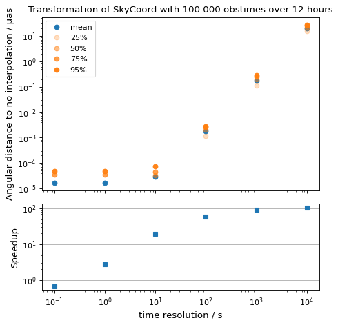
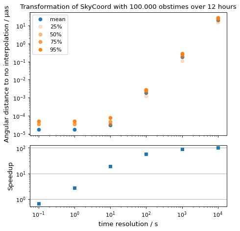
Here, we look into choosing an appropriate time_resolution.
We will transform a single sky coordinate for lots of observation times from
ICRS to AltAz and evaluate precision and runtime for different values
for time_resolution compared to the non-interpolating, default approach.
from time import perf_counter

import numpy as np
import matplotlib.pyplot as plt

from astropy.coordinates.erfa_astrom import erfa_astrom, ErfaAstromInterpolator
from astropy.coordinates import SkyCoord, EarthLocation, AltAz
from astropy.time import Time
import astropy.units as u

rng = np.random.default_rng(1337)

# 100_000 times randomly distributed over 12 hours
t = Time('2020-01-01T20:00:00') + rng.uniform(0, 1, 10_000) * u.hour

location = EarthLocation(
    lon=-17.89 * u.deg, lat=28.76 * u.deg, height=2200 * u.m
)

# A celestial object in ICRS
crab = SkyCoord.from_name("Crab Nebula")

# target horizontal coordinate frame
altaz = AltAz(obstime=t, location=location)


# the reference transform using no interpolation
t0 = perf_counter()
no_interp = crab.transform_to(altaz)
reference = perf_counter() - t0
print(f'No Interpolation took {reference:.4f} s')


# now the interpolating approach for different time resolutions
resolutions = 10.0**np.arange(-1, 5) * u.s
times = []
seps = []

for resolution in resolutions:
    with erfa_astrom.set(ErfaAstromInterpolator(resolution)):
        t0 = perf_counter()
        interp = crab.transform_to(altaz)
        duration = perf_counter() - t0

    print(
        f'Interpolation with {resolution.value: 9.1f} {str(resolution.unit)}'
        f' resolution took {duration:.4f} s'
        f' ({reference / duration:5.1f}x faster) '
    )
    seps.append(no_interp.separation(interp))
    times.append(duration)

seps = u.Quantity(seps)

fig = plt.figure()

ax1, ax2 = fig.subplots(2, 1, gridspec_kw={'height_ratios': [2, 1]}, sharex=True)

ax1.plot(
    resolutions.to_value(u.s),
    seps.mean(axis=1).to_value(u.microarcsecond),
    'o', label='mean',
)

for p in [25, 50, 75, 95]:
    ax1.plot(
        resolutions.to_value(u.s),
        np.percentile(seps.to_value(u.microarcsecond), p, axis=1),
        'o', label=f'{p}%', color='C1', alpha=p / 100,
    )

ax1.set_title('Transformation of SkyCoord with 100.000 obstimes over 12 hours')

ax1.legend()
ax1.set_xscale('log')
ax1.set_yscale('log')
ax1.set_ylabel('Angular distance to no interpolation / µas')

ax2.plot(resolutions.to_value(u.s), reference / np.array(times), 's')
ax2.set_yscale('log')
ax2.set_ylabel('Speedup')
ax2.set_xlabel('time resolution / s')

ax2.yaxis.grid()
fig.tight_layout()
See Also#
Some references that are particularly useful in understanding subtleties of the coordinate systems implemented here include:
- USNO Circular 179
A useful guide to the IAU 2000/2003 work surrounding ICRS/IERS/CIRS and related problems in precision coordinate system work.
- Standards Of Fundamental Astronomy
The definitive implementation of IAU-defined algorithms. The “SOFA Tools for Earth Attitude” document is particularly valuable for understanding the latest IAU standards in detail.
- IERS Conventions (2010)
An exhaustive reference covering the ITRS, the IAU2000 celestial coordinates framework, and other related details of modern coordinate conventions.
- Meeus, J. “Astronomical Algorithms”
A valuable text describing details of a wide range of coordinate-related problems and concepts.
- Revisiting Spacetrack Report #3
A discussion of the simplified general perturbation (SGP) for satellite orbits, with a description of the True Equator Mean Equinox (TEME) coordinate frame.
Built-in Frames and Transformations#
The diagram below shows all of the built in coordinate systems, their aliases (useful for converting other coordinates to them using attribute-style access) and the pre-defined transformations between them. The user is free to override any of these transformations by defining new transformations between these systems, but the pre-defined transformations should be sufficient for typical usage.
The color of an edge in the graph (i.e., the transformations between two frames) is set by the type of transformation; the legend box defines the mapping from transform class name to color.
-
AffineTransform: ➝
-
FunctionTransform: ➝
-
FunctionTransformWithFiniteDifference: ➝
-
StaticMatrixTransform: ➝
-
DynamicMatrixTransform: ➝
Built-in Frame Classes#
A coordinate or frame in the ICRS system. |
|
A coordinate or frame in the FK5 system. |
|
A coordinate or frame in the FK4 system. |
|
A coordinate or frame in the FK4 system, but with the E-terms of aberration removed. |
|
A coordinate or frame in the Galactic coordinate system. |
|
A coordinate or frame in the Galactocentric system. |
|
Supergalactic Coordinates (see Lahav et al. |
|
A coordinate or frame in the Altitude-Azimuth system (Horizontal coordinates) with respect to the WGS84 ellipsoid. |
|
A coordinate or frame in the Hour Angle-Declination system (Equatorial coordinates) with respect to the WGS84 ellipsoid. |
|
A coordinate or frame in the Geocentric Celestial Reference System (GCRS). |
|
A coordinate or frame in the Celestial Intermediate Reference System (CIRS). |
|
A coordinate or frame in the International Terrestrial Reference System (ITRS). |
|
A coordinate or frame in a Heliocentric system, with axes aligned to ICRS. |
|
A coordinate or frame in the True Equator Mean Equinox frame (TEME). |
|
An equatorial coordinate or frame using the True Equator and True Equinox (TETE). |
|
A coordinate frame defined in a similar manner as GCRS, but precessed to a requested (mean) equinox. |
|
Geocentric mean ecliptic coordinates. |
|
Barycentric mean ecliptic coordinates. |
|
Heliocentric mean ecliptic coordinates. |
|
Geocentric true ecliptic coordinates. |
|
Barycentric true ecliptic coordinates. |
|
Heliocentric true ecliptic coordinates. |
|
Heliocentric mean (IAU 1976) ecliptic coordinates. |
|
Barycentric ecliptic coordinates with custom obliquity. |
|
A coordinate or frame in the Local Standard of Rest (LSR). |
|
A coordinate or frame in the Kinematic Local Standard of Rest (LSR). |
|
A coordinate or frame in the Dynamical Local Standard of Rest (LSRD). |
|
A coordinate or frame in the Local Standard of Rest (LSR), axis-aligned to the Galactic frame. |